Excel Inventory Management Formulas: A Practical Guide

Understanding inventory management formulas is crucial for balancing stock levels. By calculating key figures like the Economic Order Quantity (EOQ) or your Reorder Point (ROP) directly in Excel, you can move from guesswork to making smart, data-backed decisions. This practical approach helps prevent common problems like stockouts or overstocked shelves, turning your spreadsheet into a powerful tool for financial health.

This guide will walk you through the essential inventory management formulas, providing practical explanations and actionable examples in Excel. You'll learn not just what these formulas are, but how to use them to solve real-world business problems, enhanced with tips on leveraging AI to streamline the entire process.

Why Mastering Inventory Formulas in Excel is a Game Changer

Effective inventory management is the key to healthy cash flow and a competitive edge. Without a solid system, you risk tying up capital in slow-moving products or losing sales from stockouts. This is where a firm grasp of core inventory management formulas, applied within Excel, becomes a business superpower.

By bringing these calculations into Excel, you transform a simple spreadsheet into a command center for your operations. For example, knowing your exact Reorder Point helps you avoid last-minute rush orders. Calculating your Inventory Turnover Ratio reveals which products are driving profit and which are just taking up space. The goal is to build an intelligent, responsive system that keeps supply and demand in perfect harmony.

To get started, let's create a quick reference of the essential formulas we'll be covering. This table provides a snapshot of what each formula does and the data you'll need to calculate it in Excel.

Essential Inventory Formulas at a Glance

Formula Name	Primary Purpose	Key Variables Needed in Excel
Economic Order Quantity (EOQ)	Determines the ideal order size to minimize holding and ordering costs.	Annual Demand, Order Cost, Holding Cost
Reorder Point (ROP)	Calculates the stock level at which a new order should be placed.	Lead Time Demand, Safety Stock
Safety Stock	Calculates the extra inventory needed to prevent stockouts from demand or lead time variability.	Max Daily Usage, Avg Daily Usage, Max Lead Time, Avg Lead time
Inventory Turnover Ratio	Measures how many times inventory is sold or used in a given period.	Cost of Goods Sold (COGS), Average Inventory
Days of Inventory Outstanding	Shows the average number of days a company holds its inventory before selling it.	Average Inventory, COGS, Number of Days

This table serves as a handy cheat sheet as you work through the detailed, practical examples for each formula later in this guide.

Here's a visual breakdown of the three most fundamental calculations: EOQ, Reorder Point, and Safety Stock.

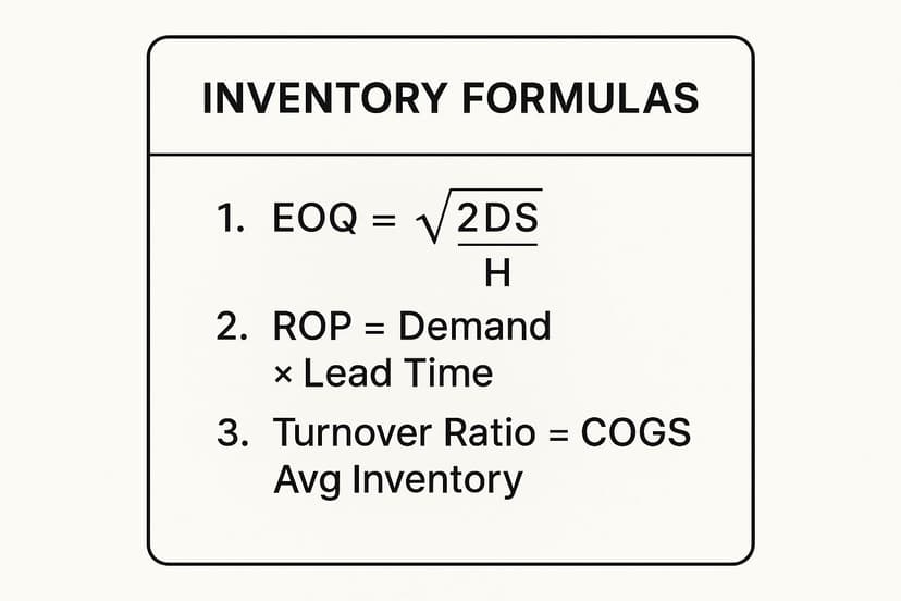
This image helps clarify how each formula plays a distinct role: EOQ tells you how much to order, the Reorder Point tells you when to order, and Safety Stock provides a crucial buffer for unexpected events.

Bringing Formulas to Life in Excel with AI

While Excel is powerful, writing and managing these formulas can be time-consuming. This is where artificial intelligence tools integrated with Excel, like Elyx.AI, change the game. Instead of wrestling with nested functions, you can simply describe the calculation you need in plain English. For example, an AI-powered Excel formula builder can generate the correct syntax for you, speeding up your workflow and reducing errors.

To truly optimize your stock, you'll want to combine these formulas with essential inventory management techniques. By weaving these calculations into your daily Excel-based operations, you shift from reacting to inventory problems to proactively managing your stock with data-driven clarity.

This guide will walk you through each formula step-by-step, complete with real-world Excel examples and actionable tips for using AI to make the process even more efficient.

Calculate Economic Order Quantity (EOQ) in Excel

The Economic Order Quantity (EOQ) is a foundational formula for any inventory manager. Its purpose is to solve a specific problem: finding the perfect order quantity that minimizes your total inventory costs, including both ordering and storage fees.

Ordering too much at once ties up capital and increases warehousing costs. Ordering too little, too often, results in high shipping and administrative fees. EOQ provides the mathematical "sweet spot" that balances these two costs, helping you run a leaner, more efficient operation.

Understanding the EOQ Formula Components

Before building the formula in Excel, let's break down its three core components. Accurate inputs are essential for a reliable result.

Annual Demand (D): The total number of units you expect to sell in a year. This figure should be based on your sales forecast.
Ordering Cost (K): The fixed cost incurred every time you place an order. This includes shipping fees, order processing costs, and related labor—not the cost of the goods themselves.
Holding Cost (H): The cost to store one unit of inventory for an entire year. This includes warehouse rent, insurance, potential spoilage, and the opportunity cost of capital.

The Economic Order Quantity formula was first developed by Ford W. Harris in 1913, and its long-standing use is a testament to its effectiveness. You can explore the history of this foundational formula to understand its impact on modern logistics.

How to Calculate EOQ in Excel: A Practical Example

Let's solve a concrete problem. Imagine you run a business selling custom-printed t-shirts. Here’s how you would calculate your EOQ in Excel to optimize your ordering process.

Set Up Your Data in Excel
First, open a worksheet and clearly label your input cells. This practice makes your spreadsheet easy to understand and update.
- A2: Annual Demand (D)
- A3: Ordering Cost per Order (K)
- A4: Holding Cost per Unit (H)
Input Your Values
Next, enter the specific data for your t-shirt business.
- B2: 1200 (You sell 100 shirts a month, so 100 * 12 = 1200)
- B3: 50 (Each order costs $50 in shipping and admin fees)
- B4: 3 (It costs $3 per year to store one t-shirt)
Build the Formula
The mathematical formula for EOQ is √((2 * D * K) / H). In Excel, you use the SQRT function to perform the square root calculation. In an empty cell, like B6, type the following:

=SQRT((2*B2*B3)/B4)

After pressing Enter, Excel will display the result: 200. This number is your actionable solution. It means the most cost-effective strategy is to order 200 t-shirts at a time, minimizing your combined annual ordering and holding costs.

AI-Powered Forecasting with Elyx.AI: An EOQ calculation is only as good as its demand forecast. Using a static number for annual demand can be a bit of a gamble. With an AI tool like Elyx.AI, you can analyze your historical sales data right inside Excel to generate a much more accurate and dynamic forecast, making your EOQ truly responsive to your business.

Implement the Reorder Point ROP Formula in Excel

While EOQ tells you how much to order, the Reorder Point (ROP) formula answers the critical question of when to order. Its sole purpose is to prevent stockouts by triggering a replenishment order before your inventory runs out. Think of it as your inventory’s automated low-fuel warning.

ROP identifies the specific stock level that should initiate your reordering process, ensuring new inventory arrives just in time. Mastering this calculation is essential for maintaining a smooth supply chain, keeping customers satisfied, and avoiding lost sales due to out-of-stock situations.

The Reorder Point Formula Explained

The standard ROP formula is straightforward, relying on two key pieces of information to determine the perfect time to reorder.

Average Daily Usage: The average number of units you sell each day. To calculate this in Excel, you can use the AVERAGE function on your daily sales data.
Lead Time: The number of days it takes for an order to arrive from your supplier after it has been placed.

The basic ROP calculation is:

Reorder Point = Average Daily Usage × Lead Time in Days

Most businesses also incorporate a safety stock buffer (which we will cover next). In that case, the formula is adjusted: ROP = (Average Daily Usage × Lead Time) + Safety Stock. For now, let's focus on the basic version.

Calculating ROP in an Excel Spreadsheet: A Step-by-Step Example

Let's solve a practical problem for a coffee shop needing to determine the reorder point for its best-selling coffee beans.

Organize Your Data in Excel: Open a worksheet and create clear labels for your inputs.
- A2: Average Daily Usage
- A3: Lead Time (in days)
Enter Your Values: Now, input the data for your coffee beans.
- B2: 10 (You sell an average of 10 bags of coffee per day)
- B3: 5 (It takes your supplier 5 days to deliver a new shipment)
Implement the ROP Formula: In another cell, such as B5, you can now calculate the reorder point.
- Type the formula: =B2*B3

Press Enter, and Excel provides the answer: 50. This is your actionable trigger point. You need to place a new order with your supplier the moment your inventory of coffee beans drops to 50 bags. This timing ensures new stock arrives just before you sell out.

The concept of timing orders has been a cornerstone of supply chain management for over a century. As logistics evolved, inventory management formulas like ROP became essential for managing complex supply networks. You can learn more about how these historical developments shaped modern inventory systems to see how their principles are still applied today.

Determine Your Safety Stock Level in Excel

The reorder point tells you when to order under normal conditions, but safety stock provides a cushion for when things go wrong. Think of it as your inventory's insurance policy, designed to solve the problem of uncertainty. It's the extra stock you hold to protect against two main risks: unexpected surges in customer demand and unforeseen supplier delays.

Without this buffer, a sudden viral trend or a shipping delay could lead to a stockout, resulting in lost sales and frustrated customers. Calculating your safety stock in Excel allows you to fulfill orders reliably, even when faced with unpredictability. It's a strategic defense against uncertainty.

Calculating Safety Stock in Excel: A Practical Method

While there are several methods to calculate safety stock, a reliable approach is to analyze the variability in both your sales and lead times. This helps you prepare for a worst-case scenario.

You will need four key data points:

Maximum Daily Sales: The highest number of units sold in a single day.
Average Daily Sales: The typical number of units sold per day.
Maximum Lead Time: The longest time it has ever taken for a supplier shipment to arrive.
Average Lead Time: The usual delivery timeframe from your supplier.

Let’s solve a problem for a business selling high-end headphones.

Lay out your data in Excel:
- A2: Maximum Daily Sales (40)
- A3: Average Daily Sales (25)
- A4: Maximum Lead Time (days) (10)
- A5: Average Lead Time (days) (7)
Enter the Safety Stock Formula:
The formula is: (Maximum Daily Sales × Maximum Lead Time) – (Average Daily Sales × Average Lead Time).
In a blank cell, such as B7, type this directly into Excel:
=(A2*A4)-(A3*A5)

Press Enter, and Excel returns the answer: 175 units. This is your safety net. You should aim to keep an additional 175 headphones in inventory to cover unexpected disruptions without stocking out.

The Strategic Value of Safety Stock

Optimizing safety stock is a balancing act. Too much, and you tie up valuable capital. Too little, and you risk stockouts. For businesses in volatile markets, safety stock can represent 20-30% of total inventory. By mastering both reorder point and safety stock calculations, companies often reduce overall inventory costs by 10-20% while significantly improving customer service levels. To see how these calculations are applied at a larger scale, you can discover more insights on Kleene.ai.

AI-Driven Safety Stock Optimization: A static safety stock calculation can quickly become outdated. AI tools like Elyx.AI can continuously analyze your sales and supplier data in real-time directly within Excel. The AI can then suggest dynamic adjustments to your safety stock, ensuring your buffer is optimized for current market conditions, not last quarter's. This provides a more intelligent and responsive solution.

How to Calculate Key Performance Indicators in Excel

While formulas like EOQ and ROP optimize your ordering process, they don't provide a complete financial overview. To understand the financial health of your inventory, you need to calculate Key Performance Indicators (KPIs). These metrics help answer a critical question: How efficiently is your inventory being converted into cash?

By calculating these KPIs in Excel, you gain the clarity needed to make smarter financial decisions, identifying whether your capital is working for you or simply sitting on a shelf.

Inventory Turnover Ratio

The Inventory Turnover Ratio is a crucial KPI that measures how many times you sell and replace your entire inventory over a specific period. A high ratio typically indicates strong sales and efficient management, while a low ratio can signal overstocking or poor sales performance.

To calculate this, you need two figures from your financial statements:

Cost of Goods Sold (COGS): The total direct cost of the products you sold, found on your income statement.
Average Inventory: The average value of your inventory over the same period. Calculate this by adding the beginning and ending inventory values and dividing by two.

Here is a practical example in Excel. Assume your COGS for the last year was $200,000, and your average inventory value was $40,000.

Set up your spreadsheet:
- In cell A2, label it "COGS" and enter 200000 in B2.
- In cell A3, label it "Average Inventory" and enter 40000 in B3.
Enter the formula: The calculation is COGS / Average Inventory.
- In a new cell, like B5, type =B2/B3 and press Enter.

The result is 5. This means your business sold through its entire inventory five times last year. This single metric provides a powerful insight into your financial efficiency. To make this data even more useful, you can learn how to create a KPI dashboard in Excel to visualize your performance over time.

Days of Inventory Outstanding (DIO)

While turnover shows how often you sell your stock, Days of Inventory Outstanding (DIO) reveals how long it sits in your warehouse before being sold. This metric, also known as Days Sales of Inventory (DSI), translates the turnover ratio into a more tangible number: days. A lower DIO is generally better, as it indicates you are converting inventory into cash more quickly.

The formula for DIO is:

(Average Inventory / COGS) * Number of Days in Period

Using the same data as before and assuming a 365-day period:

Lay out the data in Excel:
- A2: Average Inventory (40000)
- A3: COGS (200000)
- A4: Days in Period (365)
Calculate it:
- In a cell like B6, type the formula =(A2/A3)*A4.

The result is 73 days. This tells you that, on average, your inventory takes 73 days to sell. Tracking DIO in Excel is a practical way to identify slow-moving products and improve your cash flow.

Build a Dynamic Inventory Dashboard in Excel

After mastering individual calculations, the next step is to integrate them into a dynamic inventory dashboard. This transforms Excel from a simple calculator into a live command center for your business, providing a clear, visual snapshot of your inventory health. A well-designed dashboard allows you to see all your key metrics at a glance, enabling faster, more informed decisions.

The dashboard connects your raw data, cost inputs, and inventory management formulas into a cohesive system. Instead of manually recalculating every time a sale is made, the dashboard updates automatically, giving you a real-time view of what to order, when to order, and how your inventory is performing financially.

Structuring Your Excel Workbook for a Dashboard

For an effective and manageable dashboard, it's best practice to separate your data, calculations, and presentation into different worksheets. This organizational structure is a key to success.

Data Sheet: This sheet is your single source of truth, containing all raw data like daily sales, stock deliveries, and supplier lead times.
Calculation Sheet: This is the engine room where all your inventory management formulas reside. It pulls data from the "Data Sheet" to continuously recalculate EOQ, reorder points, safety stock, and KPIs.
Dashboard Sheet: This is the final presentation layer, featuring charts, KPI cards, and key figures that pull their values from the "Calculation Sheet."

This separated structure makes your workbook cleaner, reduces the risk of errors, and simplifies troubleshooting.

Integrating Formulas for a Cohesive View

The power of a dashboard lies in its interconnected formulas. Each calculation should be linked to your live data source, not static numbers. For example, your Reorder Point formula, = (Average Daily Usage * Lead Time) + Safety Stock, should have an "Average Daily Usage" component that is itself a formula, like =AVERAGE(DataSheet!C:C), actively calculating from your sales data.

When all formulas are interconnected, your dashboard becomes truly dynamic. Add new sales data, and every related metric—from reorder points to inventory turnover—updates instantly. If you are new to creating such tools, our comprehensive Excel dashboard tutorial provides a step-by-step guide.

Here's a quick reference on how to implement key formulas directly into your dashboard for actionable insights.

Implementing Formulas in Your Excel Dashboard

Metric/Formula	Excel Function/Formula Example	Dashboard Purpose	AI Enhancement
Reorder Point (ROP)	`= (AVERAGE(SalesData[Units]) * LeadTime) + SafetyStock`	Triggers an alert when a product's stock level hits the ROP.	Ask AI to "Flag all items below their reorder point in red."
Economic Order Quantity (EOQ)	`= SQRT((2 * D2 * S2) / H2)`	Provides the ideal order size to minimize holding and ordering costs.	Use AI to "Forecast next quarter's demand to get a more accurate EOQ."
Safety Stock	`= (MAX(SalesData[Units]) - AVERAGE(SalesData[Units])) * LeadTime`	Shows how much buffer stock you have to prevent stockouts.	Ask AI to "Model safety stock levels needed for a 98% service level."
Inventory Turnover	`= COGS / AVERAGE(InventoryValue)`	Measures how quickly stock is sold and replaced over a period.	Have AI "Create a trendline chart for inventory turnover over the last 12 months."

This table illustrates how each formula becomes an active component of your decision-making process, providing strategic insights rather than just static numbers.

Supercharge Your Dashboard with Elyx.AI

Building a fully interconnected dashboard in Excel can be challenging. Writing complex nested formulas and designing effective data visualizations takes time and expertise. This is where an AI assistant can be a powerful ally.

With an AI tool like Elyx.AI, you can automate much of the manual work. Simply describe the chart or metric you need in plain English, and the AI can generate the necessary PivotTable, create the graph, or write the complex formula for you.

For example, you could ask Elyx.AI: "Create a bar chart showing the current stock level vs. the reorder point for my top 10 products." The AI analyzes your data, performs the calculations, and generates the requested visual. This frees you to focus on interpreting the data and making strategic decisions, rather than getting bogged down in formula syntax.

Frequently Asked Questions

When applying inventory management formulas in Excel, several common questions arise. Here are straightforward answers to help you solve specific problems and refine your inventory strategy.

Can Small Businesses Benefit from These Formulas?

Absolutely. These formulas are highly scalable and just as valuable for a small e-commerce shop as for a large corporation. The key is to solve one problem at a time. Start by using the Reorder Point (ROP) formula in a simple spreadsheet to prevent stockouts of your best-selling product.

Once you are comfortable with that, you can implement the Economic Order Quantity (EOQ) and Safety Stock formulas to further optimize your ordering and reduce costs. Excel makes these powerful tools accessible without requiring a significant investment in specialized software.

What Are the Most Common Errors in Calculation?

The most frequent mistakes occur before the formula is even entered. Using inaccurate or outdated data is the primary cause of flawed results.

A formula is only as reliable as the data you feed it. Using a rough guess for "annual demand" or "lead time" will give you a misleading result. Always base your inputs on actual historical data for the most accurate outcomes.

Other common errors include:

Inconsistent Units: Ensure that demand, holding costs, and order costs are all based on the same time period (e.g., annual or monthly).
Ignoring Variability: Relying solely on average lead time without calculating safety stock leaves you vulnerable to stockouts from unexpected delays or demand spikes.
Forgetting "Hidden" Costs: When calculating holding costs, remember to include expenses like insurance, potential spoilage, and the opportunity cost of having capital tied up in inventory.

How Can AI Help Beyond Just Building Formulas?

While AI tools like Elyx.AI are excellent for generating complex Excel formulas from simple text prompts, their capabilities extend much further. An AI assistant can analyze your historical sales data to create a more accurate and dynamic demand forecast. This makes your EOQ and ROP calculations significantly more reliable than those based on static annual estimates.

Furthermore, AI can act as a data analyst, helping you uncover trends you might otherwise miss. You can ask it to "analyze sales data to find seasonal demand spikes for product X" or "show me which products have a declining turnover rate." This transforms your spreadsheet from a simple calculation tool into an intelligent, proactive partner for your business, helping you solve problems before they arise.

Ready to stop wrestling with complex formulas and let AI do the heavy lifting? Elyx.AI works right inside your spreadsheet, letting you generate formulas, build charts, and analyze data with simple text commands. It's time to streamline your inventory management and make smarter, data-driven decisions. Start using Elyx.AI for free.