How to Format Numbers in Excel A Practical Guide

Tired of wrestling with messy, inconsistent numbers in your spreadsheets? Here's the one shortcut every serious Excel user knows: select the cells you want to fix and hit CTRL+1 (or Cmd+1 on a Mac).

That simple command opens up the Format Cells dialog box, your central hub for turning raw data into something clear, professional, and easy to understand.

Your Quick Guide to Excel Number Formatting

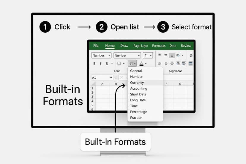
When you first pop open that Format Cells window, you'll see a list of categories on the left. These are your go-to tools for everyday data presentation. Think of them less as rules and more as different lenses to view your numbers through, each designed for a specific job.

The whole point is to get away from the default "General" format, which honestly does a poor job of interpreting what you actually mean. A sales report is instantly more readable with currency symbols, and survey results make more sense as percentages. These small tweaks prevent confusion and help people see the story in your data right away.

Core Formats and Their Purpose

Before we get into the really powerful custom stuff, you have to nail the basics. The truth is, these built-in formats will handle over 90% of what you need to do on any given day.

Currency: Perfect for financial data like budgets or sales forecasts where you need that dollar sign right next to the number.
Accounting: This one is a subtle but important variation of Currency. It perfectly aligns all the currency symbols and decimal points in a column, which makes formal financial statements look incredibly clean and professional.
Percentage: This format is a lifesaver. It instantly turns a decimal like 0.75 into 75%, which is ideal for showing things like market share, growth rates, or survey responses.
Number: Your workhorse for general numeric data. It gives you precise control over decimal places and lets you add thousand separators for readability.

The real magic of Excel formatting isn't just in the built-in options; it's in the custom syntax. This is where you can create your own rules to handle positive, negative, and zero values—all within a single format string.

For example, I often use a custom format like #,##0.0;[Red]-#,##0.0;0;@. This automatically shows any negative number in red, giving an immediate visual warning for a deficit or loss without me having to lift a finger. Once you get the hang of this, it completely changes how you build reports. If you're ready to go deeper, it's worth exploring the world of custom number formatting in Excel.

To make this all a bit easier to digest, I've put together a quick reference table of the most common formats and when I typically use them.

Common Excel Number Formats and Their Uses

Here’s a quick-glance guide to the built-in number formats you'll use most often in Excel, along with the best scenarios for each.

Format Type	What It Does	Best Used For
General	Default format with no specific rules.	Quick data entry, raw numbers.
Number	Adds decimal places and separators.	Scientific data, measurements.
Currency	Adds a currency symbol next to the number.	Budgets, invoices, price lists.
Accounting	Aligns currency symbols and decimals.	Formal financial reports, balance sheets.
Percentage	Multiplies by 100 and adds a % sign.	Market share, survey results, growth analysis.

Keep this handy as you work—soon, choosing the right format will become second nature, making your spreadsheets more powerful and much easier to read.

A Closer Look at Excel's Built-In Number Formats

When you first start working with Excel's number formats, many of them can seem pretty similar. But once you dig in, you'll find there are subtle yet important differences that can make your spreadsheets much clearer and more professional. It’s all about picking the right tool for the specific job you're doing.

Let's break down the practical distinctions that will seriously level up how you present your data.

Knowing when to use one format over another is what separates a basic spreadsheet from a polished financial report.

Currency vs. Accounting: It's All About Alignment

At a quick glance, the Currency and Accounting formats seem almost identical. They both slap a dollar sign on your numbers and manage decimal places. The real difference is alignment, and it matters more than you might think.

The Currency format tucks the dollar sign right up against the first digit. This is perfect for simple lists or compact tables where you're trying to save space.

On the other hand, the Accounting format does something really slick: it pushes all the currency symbols to the far left of the cell while also perfectly aligning every decimal point vertically. This creates an incredibly clean, uniform column that's super easy to read, which is why it's the standard for formal financial documents like balance sheets and P&L statements.

Getting Dates and Times Right

Here’s a little secret: Excel doesn't actually see dates and times the way we do. Under the hood, every date is just a serial number. For instance, Excel stores January 1, 1900, as the number 1. This is actually a feature, not a bug, as it lets you perform calculations, like figuring out the number of days between two project deadlines.

Your job is simply to apply a format that makes sense to a human eye. You’ve got a ton of built-in options to choose from:

Short Date: A classic, like 3/15/2024
Long Date: More formal, like Friday, March 15, 2024
Custom Formats: You can also create your own, such as 15-Mar or March-24.

Time works on the same principle, but it's stored as a fraction of a 24-hour day. That's how Excel can take a value like 0.75 and, with the right format, display it as 6:00 PM.

My Favorite Pro Tip: Ever see a cell filled with pound signs (######) and think you broke something? Don't worry. This almost never means your data is wrong. It's just Excel's way of saying the column is too narrow to show the fully formatted number. A quick double-click on the right-hand border of the column header will instantly fix it.

Showing Proportions with Percentage and Fraction

The Percentage format is one you'll use all the time. It’s simple but powerful. It takes a decimal like 0.25, automatically multiplies it by 100, and sticks a percent sign on the end, turning it into 25%. It's absolutely essential for showing anything from sales growth and budget variances to survey results.

The Fraction format is a bit more niche but can be a lifesaver in the right situation. If you're working with recipes that call for 1/2 a cup of something, or maybe even tracking old-school stock prices, this format will display a decimal like 0.5 as the fraction 1/2.

Getting comfortable with these built-in options ensures your data is always presented in the most logical and visually appealing way possible. This clarity becomes even more vital as your reports grow in complexity. For those who want to take it a step further, understanding Excel report automation can help you apply these formatting rules across massive datasets in an instant, saving you a huge amount of time.

Creating Custom Number Formats for Full Control

While Excel’s built-in formats get the job done for most everyday tasks, custom number formatting is where you really start to take control. This is the difference between letting Excel make the call and telling it exactly how you want your data to look. Once you understand a few simple codes, you can build formats that are perfectly tailored to your reports.

This infographic gives a great overview of how Excel’s formatting options are structured, from the basics right on the ribbon to the more advanced stuff we're about to dive into.

Think of the standard formats as your starting point. Now, let’s go behind the scenes and create our own rules.

Understanding the Core Placeholders

At the heart of every custom format are two critical symbols: the zero (0) and the pound or hash sign (#). They might seem similar, but they behave very differently, and knowing which one to use is key.

The 0 is a digit placeholder that forces a digit to be displayed. If a number doesn't have enough digits to fill the zeros in your format, Excel pads it with extra zeros. For example, using the format 000.00 on the number 7.5 would display it as 007.50.
The # is also a digit placeholder, but it only shows significant digits. It won’t display extra, non-significant zeros, keeping things looking clean. Using ###.## on that same number 7.5 would simply display 7.5.

I like to think of it this way: use the 0 when you need consistent length, like for product codes or IDs. Use the # when you want a tidier look that trims unnecessary zeros from your financial reports.

The Four-Part Format Code

The real power of custom formats comes from a hidden structure. Every custom format can have up to four sections, separated by semicolons, with each one controlling a different type of value.

The structure is: POSITIVE;NEGATIVE;ZERO;TEXT

This means you can set a unique rule for how positive numbers, negative numbers, and zeros appear, all within a single format string. You can even define how any text that lands in the cell should be displayed.

A fantastic real-world use for this is creating a financial view that automatically colors negative numbers red without messing with conditional formatting. A format like #,##0;[Red]-#,##0;0 tells Excel to show positive numbers normally, make negative numbers red with a minus sign, and display all zeros as a single 0.

Practical Recipes for Custom Formats

Alright, let's move from theory to practice. Here are some incredibly useful custom format "recipes" you can copy and paste directly into the custom format box (CTRL+1 > Custom).

Standard US Phone Number: To turn a raw number like 5551234567 into a clean (555) 123-4567, just use this format code: (###) ###-####.
Adding Text Units: If you're tracking inventory or measurements, you can add units that appear in the cell but don't affect calculations. The format # "kg" will display the number 150 as 150 kg. The text inside the quotes appears exactly as you type it.
Hiding Numbers Completely: This is a sneaky but useful one. Sometimes you need a number for a calculation, but you don't want it visible on the sheet. The format code ;;; will hide any value in the cell—positive, negative, zero, or text—while keeping it available for your formulas to reference.

To help you get started, here's a quick reference table breaking down the most common symbols you'll use to build your own custom formats.

Key Custom Format Codes Explained

Code/Symbol	Function	Example Usage
`0`	Digit placeholder; shows insignificant zeros	`0.00`
`#`	Digit placeholder; hides insignificant zeros	`#,##0.##`
`?`	Digit placeholder; adds space for insignificant zeros	`?.??` (aligns decimal points)
`.`	Decimal point	`#,##0.00`
`,`	Thousands separator	`#,##0`
`[Color]`	Applies a specific color to the section	`[Red](#,##0)`
`"text"`	Displays the exact text inside the quotes	`0 "units"`
`@`	Text placeholder	`"Name: "@`
`;`	Separator for positive, negative, zero, and text formats	`#,##0;[Red](#,##0);"-"`

Mastering these codes is a massive step toward making your spreadsheets more professional and far more intuitive. Of course, once your data is well-formatted, you might realize you also need to tidy up the raw values themselves. For more on that, check out our guide on how to clean data in Excel, which is the perfect next step after mastering your formatting.

How to Format Large Numbers for Readability

When you're building a dashboard or a high-level summary, a raw number like 14,831,922 isn't just detailed—it's distracting. Let's be honest, decision-makers don't need to see every last digit. They need to grasp the scale of the number instantly. This is where knowing how to properly format large numbers becomes a game-changer in Excel.

Instead of showing an overwhelming string of digits, a simple custom format can make your data clean, professional, and immediately understandable. The secret is using commas in your format code, but not just for separating thousands. When placed at the end of your format code, each comma effectively divides the number by 1,000.

It’s a simple trick, but it's incredibly powerful for creating reports where clarity is king.

Scaling Numbers to Thousands and Millions

Let’s take that messy 14,831,922 and turn it into something an executive can digest at a glance. To show this number in thousands, you just need a format code ending with a single comma.

For Thousands (K): In the custom format box, type #,"K". This tells Excel to divide the number by 1,000, round it, and add a "K" at the end. Our example number now reads 14,832K. Much better.

Want to take it a step further and display it in millions? Just add a second comma.

For Millions (M): Use the custom format #.#,,"M". This code divides the number by one million (that’s 1,000 times 1,000), shows it with one decimal place, and tacks on an "M". The result is a clean and simple 14.8M.

Mastering number formatting is essential when you're dealing with big datasets, particularly in finance. Turning raw figures into clean formats like millions (M) or thousands (K) instantly makes your spreadsheets look more professional and makes the data less intimidating.

Think about it: This doesn't just change how a number looks; it changes how quickly your audience can process the information. A chart with values like '$1.2M' and '$2.5M' is far more effective than one cluttered with '$1,200,000' and '$2,500,000'.

This approach is especially handy when you https://www.getelyxai.com/en/blog/create-charts-in-excel, as it keeps your axes and data labels from becoming a cluttered mess. With AI becoming more integrated into our daily tools, like Microsoft Copilot for Finance, the need for clear, well-presented data is only going to grow. By getting these formatting codes down, you ensure your reports aren't just accurate—they communicate their message with maximum impact.

Handling International Number Formatting

If you’ve ever worked on a project that crosses borders, you know how quickly a simple number can turn into a big headache. Let's say you're collaborating with teams in both Chicago and Berlin. You send over a spreadsheet with the number 1,234.56. To you, that’s clearly "one thousand, two hundred thirty-four, and fifty-six cents." But in Germany, they’ll see it as 1.234,56. Worlds apart.

This isn’t a bug—it’s actually Excel trying to be helpful. By default, it just copies whatever regional settings your computer uses for number separators. This is great for keeping things consistent locally, but it can throw a real wrench in the works when you're sharing files with an international team.

Overriding Your System's Default Separators

So, what’s the fix? You can’t exactly ask your entire global team to change their computer settings every time they open your file. The real solution is to take control of the formatting right inside Excel.

You'll find the setting tucked away in the Advanced Options menu. Just go to File > Options > Advanced. Right near the top, you'll see a little checkbox that says "Use system separators." This is the magic button.

Unchecking it unlocks the fields right below, letting you tell Excel exactly which symbol to use for decimals and which to use for thousands.

Let's stick with our example. If you're on a European computer but need to create a report for your US colleagues, you would:

Uncheck the Use system separators box.
Set the Decimal separator to a period (.).
Set the Thousand separator to a comma (,).

It’s easy to forget that these formatting differences aren't just quirks. They're tied to deep-seated cultural norms that dictate how people read and process numbers. Getting this right isn't just about good data hygiene; it's about clear communication.

Why This Matters for Global Teams

This might seem like a small detail, but in international business, the wrong separator can lead to massive data errors and costly misunderstandings. Imagine a financial model where every number is off by a factor of a thousand. Ouch.

By manually setting the separators for a specific file, you make sure your data tells the same story, no matter where in the world someone opens it. It's a simple adjustment that can prevent a world of confusion. To get a better sense of how these conventions play out globally, you can explore more on international data conventions and see why this tiny setting has such a big impact.

Answering Common Excel Formatting Questions

Even after you get the hang of the basics, Excel has a way of throwing you for a loop. Let's walk through some of the most common formatting headaches I've seen over the years and how to fix them. This is your quick-and-dirty guide for those little quirks that pop up when you least expect them.

Ever had that moment of panic when a column suddenly fills up with hashtags (######)? Don't worry, your data is safe. That's just Excel's way of telling you the column isn't wide enough to show the number you've entered. The fix is simple: just double-click the right border of the column header, and it will automatically snap to the perfect width.

Keeping Those Leading Zeros

Here’s another classic problem: you try to type in something like an employee ID (00782) or a ZIP code for New England (01234), and Excel immediately chops off the zeros, leaving you with 782. Frustrating, right? Excel assumes you're entering a number, and mathematically, those leading zeros don't mean anything.

To get around this, you have to signal to Excel that you want to treat the entry as text. The best way to handle this for a whole column is to format it as Text before you start typing. Just select the column, hit CTRL+1 to open the Format Cells window, and pick "Text" from the list.

For a one-off entry, there's an even quicker trick. Just type an apostrophe (') right before the number. So, you'd type '00782. The apostrophe won't show up in the cell, but it forces Excel to keep your leading zeros exactly as you entered them.

It's crucial to understand the difference between what a cell shows and what it contains. Formatting changes the appearance, not the underlying value. A cell displaying "$50.00" is still just the number 50 to Excel, and that's the value it uses in all your formulas.

The Best Kept Secret for Quick Formatting

Once you've spent time getting a cell's format just right—maybe a custom currency style or a specific date layout—you don't have to go through all those steps again. This is where the Format Painter becomes your absolute best friend.

You'll find it on the Home tab; it's the little paintbrush icon. Using it is a breeze:

Select the cell with the formatting you love.
Click the Format Painter icon. Your cursor will change to a paintbrush.
Now, just click and drag over any other cells you want to apply that same formatting to.

Here’s a pro tip: if you need to apply that format to a bunch of different cells or sections that aren't next to each other, double-click the Format Painter. This keeps it "active," so you can keep clicking on cells to paste the format. When you're done, just hit the Escape key to turn it off. It’s a massive time-saver for making your spreadsheets look consistent.

Tired of fighting with tedious Excel tasks? Elyx.AI plugs directly into your spreadsheet, letting you clean up data, write formulas, and find insights just by typing what you need. Change how you work and really tap into your data's potential. Visit the Elyx.AI website to get started.