How to Clean Data in Excel Like a Pro

Let's get one thing straight: raw data is almost always messy. Before we jump into the nitty-gritty of how to clean data in Excel, it’s crucial to talk about why it matters so much. Dirty data isn't just a small annoyance; it's a genuine threat to accurate analysis and smart business decisions.

Think about it. What if you're pulling together a sales report, but duplicate entries are accidentally doubling your revenue figures? Or imagine launching a marketing campaign where your customer data is split across entries like "USA," "U.S.," and "United States." Your targeting would be a mess. These aren’t just hypotheticals—they are real, everyday problems that cost companies serious time and money.

The Real Cost of Messy Data

Sloppy data creates a ripple effect, undermining everything from simple reports to major strategic initiatives. It's why data professionals spend so much of their time just prepping data before the real analysis can even begin.

In fact, poor data quality is a major headache for analysts everywhere. Research reveals that about 20% of IT and data professionals cite poor data quality as a primary challenge, which directly sabotages the accuracy of their work. You can dig deeper into these findings by exploring common data quality challenges in survey research.

This is where data cleaning becomes your most valuable first step.

As you can see, the process is all about turning unreliable raw information into a trustworthy asset. This clean foundation is what fuels better decision-making and keeps operations running smoothly.

Data cleaning isn't just about deleting a few rows or fixing typos. It's about building a foundation of trust in your data. It ensures that every chart, pivot table, and insight you create is based on reality, not on hidden errors.

Common Data Messes and Their Business Impact

I've seen these issues pop up time and time again. Here’s a quick rundown of the usual suspects and the trouble they can cause.

Data Issue	Example	Potential Business Impact
Duplicate Records	The same customer is listed twice with slightly different names.	Inflated customer counts, skewed sales metrics, and wasted marketing spend.
Formatting Errors	Dates are mixed between "MM/DD/YYYY" and "DD-Mon-YY".	Inability to sort or filter chronologically, leading to incorrect trend analysis.
Structural Mistakes	Extra spaces before or after a product name (" Widget" vs. "Widget").	VLOOKUPs and other functions fail, breaking reports and dashboards.
Inconsistent Casing	"New York," "new york," and "NEW YORK" in the same column.	Data gets incorrectly grouped, making geographic analysis unreliable.
Missing Values	Blank cells in a 'Revenue' or 'Quantity' column.	Skewed averages and totals, potentially leading to flawed financial forecasting.

These small inconsistencies might seem minor, but they add up, creating a foundation of bad data that can lead to bad decisions.

Getting a handle on a few key data cleaning techniques in Excel elevates you from a simple spreadsheet user to a data gatekeeper. You become the person who protects the integrity of your company's information. The main culprits you’ll be fighting off are:

Duplicate Records: Redundant entries that bloat your datasets and throw off metrics.
Formatting Errors: Inconsistent dates, numbers, and text that break formulas and sorting.
Structural Mistakes: Hidden spaces or funky characters that trip up filters and lookups.
Missing Values: Blank cells that can cause calculations to fail or produce misleading results.

Your First Steps in Practical Data Cleaning

Alright, let's roll up our sleeves and get into the nitty-gritty. We're going to tackle the most common data messes you’ll run into in the real world. Getting these fundamentals right is the bedrock of any reliable analysis, so we'll start with the basics that deliver the biggest impact.

The first, and maybe the most frequent, headache is duplicate records. Imagine a customer list where "John Smith," "J. Smith," and "john smith" are all separate entries for the same person. These little redundancies can seriously inflate your customer count and throw your sales figures way off.

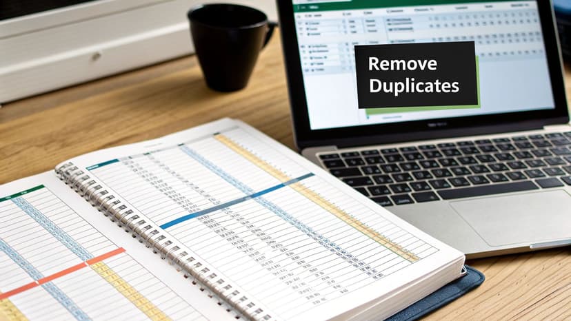
Excel has a built-in tool for this. Just select your data, head to the Data tab, and click Remove Duplicates. It’s a fast, one-click fix, but be careful—it's permanent. I always, always work on a copy of my data before doing something this drastic.

A Smarter Way to Handle Duplicates

Sometimes, just blasting away duplicates isn’t the right move. What if those "duplicate" rows have slightly different, but still important, information in other columns? A much safer approach is to highlight them first so you can give them a quick manual review.

Here’s my go-to method for this:

Select the column you want to check, like an 'Email' or 'Customer ID' column.
On the Home tab, find Conditional Formatting, then go to Highlight Cells Rules > Duplicate Values.
Pick a color, and Excel will instantly light up every single duplicate cell for you.

This simple visual cue lets you inspect each potential duplicate pair and make an informed decision. You get to decide what to keep and what to merge, rather than letting Excel make the choice for you. This technique has saved me from accidentally deleting valuable data more times than I can count.

It’s no surprise that managing duplicates and fixing missing values account for over 50% of the most common data cleaning tasks in Excel. Clean data isn't just a "nice-to-have"; it's essential for any meaningful analysis downstream.

Fixing Annoying Structural Errors

Duplicates are just one piece of the puzzle. You also have to deal with structural errors—things like extra spaces or inconsistent capitalization that can quietly break your formulas and mess up your sorting. Let’s use a messy contact list as our example to fix these frustrating issues.

Have you ever had a VLOOKUP fail for no apparent reason? Hidden leading or trailing spaces are often the culprit. You’ll see " Jane Doe " instead of "Jane Doe," and Excel treats them as completely different. The TRIM function is your best friend here.

My trick is to create a temporary column right next to the messy one. In the first cell, just type =TRIM(A2) (assuming your data starts in cell A2) and drag the formula down. The function zaps all the extra spaces, leaving just a single, clean space between words.

Next up is inconsistent capitalization. Think "new york," "New York," and "NEW YORK" all in the same column. It makes grouping and filtering a nightmare. For this, I turn to the PROPER function. Using =PROPER(B2) will instantly convert your text to proper case, capitalizing the first letter of each word. So much cleaner.

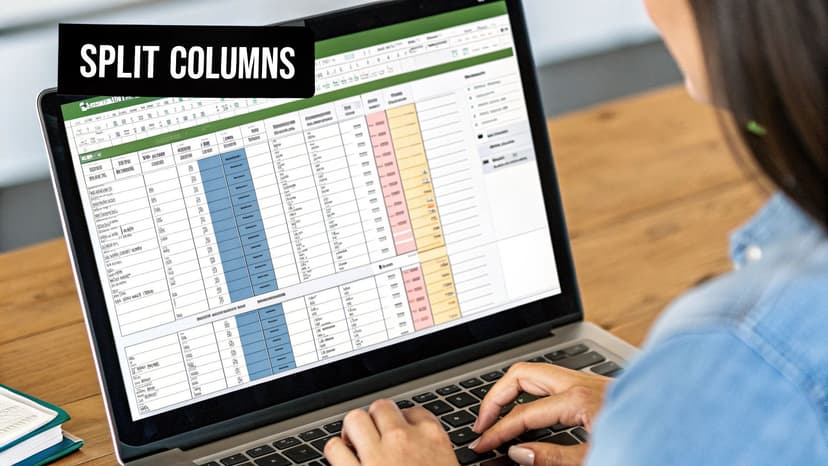
Finally, what about when an entire address is crammed into one cell, like "123 Main St, Anytown, CA, 90210"? You can't analyze data by city or state when it's all jumbled together. This is where Text to Columns is a lifesaver.

Select the column, go to Data > Text to Columns, and a handy wizard will pop up. You can tell it to split the text into new columns based on a delimiter, like a comma. In a few clicks, you’ve transformed one useless column into several clean, structured ones.

Once your data is this clean, you'll be ready for the fun part. Check out our guide on how to analyze data in Excel to see what you can do next.

Standardize Your Data for Total Consistency

So, you've wrangled the extra spaces and fixed the weird capitalization. That's a great start. But the next hurdle, standardization, is where many data cleaning efforts fall short. Inconsistent entries are sneaky—they can quietly wreck your analysis, leading to skewed pivot tables and formulas that just don't work. For your results to be trustworthy, uniformity is non-negotiable.

Think about it. You're trying to pull a sales report, but your country column has "USA," "U.S.," and "United States." To you and me, that's all the same place. But to Excel, they're three completely different categories. This common problem splinters your data, making it impossible to group and analyze anything accurately.

Luckily, there's a quick fix for this: Find and Replace.

Just hit Ctrl + H to bring up the tool. From there, you can hunt down each variation like "U.S." and replace it with your chosen standard, like "United States." It’s a simple move, but it’s incredibly effective for bringing your text-based data into alignment.

Standardizing Formats for Flawless Calculations

It’s not just text that causes headaches. Numbers and dates can be just as chaotic. I’ve seen spreadsheets where one column has dates like "10/25/2024," "25-Oct-24," and even "October 25, 2024." When that happens, Excel gets confused and might not recognize them all as dates, completely breaking any sorting or calculations based on time.

To get everything on the same page, just highlight the column, right-click, and choose Format Cells. You can then pick a single, consistent format—I personally prefer MM/DD/YYYY for clarity—and apply it to everything at once. This forces Excel to see every entry correctly, which stops those frustrating errors in their tracks. The same principle works wonders for currency, percentages, and other numbers.

The best data cleaning strategy? Prevent the mess from ever happening. While fixing existing issues is a necessary skill, building safeguards into your spreadsheets from the get-go saves a ton of time and ensures your data is reliable from the moment it's entered.

Preventing Errors with Data Validation

If you want to move from reactive cleaning to proactive data management, Data Validation is your best friend. Instead of endlessly fixing the same old mistakes, you can set up rules that prevent them from being entered in the first place.

My favorite way to use this is by creating dropdown lists. For that country column we talked about, why let people type anything they want? Instead, give them a predefined list: "United States," "Canada," "Mexico." This simple step eliminates typos and variations entirely.

Here’s the game plan for setting it up:

First, create your master list. Put your approved entries (like your list of countries) in a column somewhere, maybe on a hidden sheet.
Next, select the cells where you want the dropdown to appear.
Then, head to the Data tab and click on Data Validation.
In the settings, under the "Allow" dropdown, select List.
For the "Source" field, simply select the range of cells that holds your master list.

And that's it. Now, anyone entering data in that column has to pick from your approved options. Consistency guaranteed.

Once your data is this clean and standardized, you're ready to create some powerful visuals. To learn how to turn your pristine data into compelling charts, take a look at our guide on data visualization best practices.

Automate Your Workflow with Power Query

So far, we've walked through some powerful but manual fixes—using built-in tools and functions to clean up a messy spreadsheet. That's a crucial skill, but what about the reports you get every single week? The ones that are always messy in the same way? Repeating those cleanup steps over and over isn't just mind-numbing; it's a perfect recipe for mistakes.

If you're tired of doing the same tedious cleanup, it's time to meet Power Query. It’s Excel’s own data transformation engine, and while it sounds a bit technical, it’s surprisingly approachable. Think of it as a macro recorder specifically for data cleaning—it watches every step you take and can replay them flawlessly whenever you need.

Your First Power Query Project

Let's ground this in a real-world scenario I see all the time. Imagine it's Monday morning, and you've just downloaded the weekly sales export. It’s a CSV file, and it's always a mess—packed with extra columns, inconsistent text formats, and a few rogue error rows. Instead of cleaning it by hand again, we're going to build a reusable cleaning "recipe" with Power Query.

To get started, head to the Data tab in Excel. In the "Get & Transform Data" group, click From Text/CSV. Once you select your messy file, Excel does something different. Instead of just dumping the data into a sheet, it launches the Power Query Editor.

This is a separate, dedicated window where all the magic happens. Your data is staged here for cleaning before it ever touches your spreadsheet.

The editor gives you a clean preview of your data and a ribbon full of user-friendly cleaning tools. No complex formulas needed.

Inside the editor, you can perform all the usual cleaning tasks with a few simple clicks:

Remove Columns: Don't need a specific column? Just right-click its header and select "Remove."
Filter Rows: Use the filter arrows on any column to get rid of rows with errors or null values, just like you would in a regular Excel table.
Replace Values: Right-click a column and choose "Replace Values" to standardize your text, like changing every "N/A" to "0".
Change Data Types: Click the little icon in the column header (like ABC or 123) to set the correct data type. This is how you ensure numbers are treated as numbers and dates are recognized as dates.

The Magic of Repeatable Steps

Now, here's where Power Query really changes the game.

Look over to the right side of the Power Query Editor, and you'll find a panel called "Applied Steps." Every single action you take—removing a column, filtering a row, changing a format—gets recorded here as a neat, sequential step.

Power Query doesn't just clean your data once; it builds a repeatable, automated process. You are essentially creating a custom data cleaning machine that you can run again and again with a single click.

Once you’re happy with how the data looks, click "Close & Load." Power Query will then load your perfectly cleaned data into a new sheet in your workbook.

The real payoff comes next week. When you get the new messy CSV, just save it over the old one (using the exact same file name and location). Now, open your Excel workbook, go to the Data tab, and click Refresh All.

In seconds, Power Query re-runs every single one of your recorded steps on the new data. It removes the same columns, applies the same filters, and fixes the same formats automatically. Your table updates with the new, perfectly cleaned data. Just like that, you've reclaimed hours of your week and guaranteed 100% consistency in your reports.

For recurring tasks, automating with Power Query is a clear winner over manual methods. The initial setup takes a few minutes, but the long-term benefits in time savings and accuracy are massive.

Manual Cleaning vs Power Query Automation

Feature	Manual Cleaning in Excel	Automated Cleaning with Power Query
Repeatability	Low. Steps must be redone for each new file.	High. Create the process once, refresh with one click.
Accuracy	Prone to human error. Easy to miss a step or make a mistake.	Consistent. The exact same steps are applied perfectly every time.
Time Investment	High. Time-consuming, especially with large datasets.	Low (after setup). Initial setup required, then seconds to refresh.
Audit Trail	None. No record of what changes were made.	Built-in. The "Applied Steps" pane shows every transformation.
Data Source	Destructive. Original messy data is often overwritten.	Non-destructive. The original source file remains untouched.

Ultimately, by shifting from one-off manual fixes to an automated Power Query workflow, you’re not just learning another Excel feature. You're adopting a smarter, more reliable, and far more efficient approach to managing your data.

Smart Ways to Handle Missing Data

An empty cell is more than just a blank space; it’s a hole in your data's story. How you decide to fill that gap—or if you fill it at all—can dramatically change the outcome of your analysis. Missing values aren't just an annoyance. They can break formulas, throw off averages, and seriously damage the credibility of your work. Getting good at handling them is a fundamental skill for anyone working with data in Excel.

Instead of scrolling endlessly hunting for blank cells, there's a much faster way. Excel’s Go To Special feature is a lifesaver here. Just highlight your data range, press F5 to pop open the "Go To" box, click the "Special…" button, and choose "Blanks." Just like that, every single empty cell in your selection is highlighted, ready for you to make a move.

Choosing Your Strategy for Blanks

With all your blanks selected, you’re at a crossroads. What’s the right call? The answer really depends on the story your data is telling and what you need it to do next.

Here are the common plays I see, each with its own pros and cons:

Delete the entire row: This is the nuclear option. It’s really only a good idea if a row is completely useless without the missing piece of information. Be careful with this one—you could easily throw away perfectly good data from other columns.
Fill with zero (0): This is a popular choice for numerical columns, but it's a dangerous one. Dropping a zero into a blank cell will drag down your averages and sums. Only do this if a blank genuinely means "zero," like for a day with no sales.
Fill with "N/A" or "Not Applicable": I’m a much bigger fan of this approach. Using a text placeholder like "N/A" clearly flags the data as missing without messing up your math. Functions like AVERAGE or SUM simply ignore the text, which is exactly what you want.
Fill with the value from the cell above: This trick is perfect for cleaning up exported reports where a category is listed once at the top of a group. It quickly turns a messy, human-readable report into a structured table ready for proper analysis.

The best way to handle missing data is always contextual. I've seen people introduce huge errors by blindly deleting rows or filling cells with zeros. Always stop and ask why a cell is blank before you decide how to fix it.

Proactively Managing Errors

Beyond just filling blanks, you can get ahead of problems by using formulas to manage potential errors. The IF and IFERROR functions are your best friends here. For instance, instead of a simple division that might blow up with a #DIV/0! error, you can wrap it in a smarter formula.

Try this: =IFERROR(A2/B2, "Invalid Data").

This formula tries to do the math. If it works, great. If it fails for any reason, it returns a clean, descriptive message like "Invalid Data" instead of a jarring error code. This keeps your calculations running and your final report looking clean and professional.

Building this solid data foundation is non-negotiable, especially when you're getting ready for more advanced analysis. For example, creating reliable pivot tables is impossible without the clean, consistent data you’ve just prepared.

FAQs: Your Data Cleaning Questions, Answered

Once you've got the basics of data cleaning down, the real-world questions start to surface. You'll find yourself wondering about the best approach for a specific problem or how to stop wasting hours fixing the same mistakes over and over. Let's dig into a few of the most common questions I get from people learning to clean data in Excel.

A big one is what to do with missing data: should you delete the row or fill the blank? Deleting an entire row is a drastic move. I only recommend it if the missing piece of information makes the rest of the data totally useless—think of a sales record that's missing the actual sale amount.

For almost everything else, filling the gap is the smarter play. Using a placeholder like "N/A" or "Not Provided" keeps all the other valuable data in that row intact. Crucially, it also prevents your formulas from throwing errors and stops your averages from being skewed by what might otherwise be treated as a zero.

Which Tool Should I Use, and When?

Another question that comes up constantly is when to use a simple Excel function versus a more robust tool like Power Query. My answer always boils down to a single factor: repetition.

If you're just tidying up a small dataset for a one-off project, built-in functions are your best friend. They're quick, easy, and get the job done for those immediate fixes. But if you find yourself cleaning the same messy report every week or every month, that’s your cue to switch to Power Query.

Setting up a cleaning workflow in Power Query might take a little time upfront, but it’s a one-time investment. After that, you can clean your entire dataset with a single click of the "Refresh" button. This not only saves you from mind-numbing repetitive tasks but also eliminates the risk of human error.

Here’s a simple way to think about it:

One-Time Cleanup: Stick with functions like TRIM, PROPER, and Find & Replace.
Recurring Cleanup: Automate your life with Power Query.

How Do I Keep My Data Clean for Good?

Fixing a dirty spreadsheet is one thing, but preventing it from getting messy in the first place is the real win. The most effective long-term strategy is all about prevention, and your best tool for this is Data Validation.

By creating dropdown lists for columns with standard entries (like "Region" or "Status"), you eliminate bad data at the source. No more hunting down typos or trying to standardize "USA" with "U.S.A." and "United States." When people have to pick from a list, the data stays perfectly consistent. This single proactive step will dramatically cut down your future cleaning time and is the key to maintaining high-quality data.

Tired of cleaning data by hand? What if AI could handle the tedious work for you? With Elyx.AI, you can clean, translate, and analyze your data using simple, natural language prompts—right inside Excel. Get your time back and make sure your data is always ready for analysis. Start your free trial of Elyx.AI today and discover just how easy data cleaning can be.