Excel Formulas for Beginners: A Practical Guide to Getting Started

Diving into Excel formulas might seem intimidating, but it's really about two key ideas: starting every formula with an equals sign (=) and using cell references instead of fixed numbers. Instead of typing =5+10, you'll use something like =A1+B1. That one small shift is the secret to creating dynamic, powerful spreadsheets that update automatically.

Your First Steps with Basic Excel Formulas

Staring at a blank grid of cells and feeling a bit lost? We’ve all been there. The great thing about Excel is that you don't need to memorize hundreds of functions to solve real-world problems. Grasping a few core concepts is enough to handle most everyday tasks.

Think of an Excel formula as a simple instruction. Every single one, no matter how basic or complex, kicks off with the equals sign (=). It’s the universal signal to Excel that says, "Okay, it's time to calculate something."

The Power of Cell References

The real game-changer is using cell references instead of just typing numbers directly into your formula. A cell reference is simply the cell's address, like A1 (column A, row 1).

So, instead of a static formula like =5+10, a much smarter approach is to put the number 5 in cell A1, 10 in cell B1, and then write your formula as =A1+B1 in a third cell, say C1.

Why does this matter so much?

It’s Dynamic: If you go back and change the value in cell A1 from 5 to 20, your total in C1 instantly updates to 30. No manual recalculation is needed.
It’s Transparent: Anyone can click on your formula and immediately see which cells are part of the calculation, making your work easy to understand and audit.
It’s Scalable: Need to perform the same calculation for an entire column of data? Just drag the formula down, and Excel handles the rest. This is a massive time-saver.

Excel formulas are the engine of any effective spreadsheet. Learning just a handful of them can completely transform how you handle routine calculations and data analysis, saving you significant time. You can discover more about the practical applications of Excel formulas and how they impact productivity.

Basic Arithmetic in Action

Let's apply this with a practical scenario: a simple budget tracker. You might have a column for income and other columns for various expenses. By using basic math operators, you can get a clear picture of your finances in seconds.

These operators are the absolute foundation for almost all excel formulas for beginners.

Before we build a formula, here’s a quick rundown of the essential operators you'll use constantly.

Core Arithmetic Operators in Excel

Operator	Name	Example Formula	What It Does
`+`	Addition	`=A1+B1`	Adds the two values
`-`	Subtraction	`=A1-B1`	Subtracts B1 from A1
`*`	Multiplication	`=A1*B1`	Multiplies the two values
`/`	Division	`=A1/B1`	Divides A1 by B1

Getting comfortable with these four symbols is the first practical step toward making Excel work for you.

The Five Essential Functions You'll Use Every Day

Once you've mastered the basic math operators, it's time to explore functions. Think of functions as pre-built shortcuts that do the heavy lifting for you. Instead of trying to learn dozens at once, we'll focus on the five true workhorses you'll find yourself using constantly.

Mastering these core functions will completely change how you work in Excel. They form the foundation for almost everything you'll do, from simple lists to more complex analysis.

The Big Three: SUM, AVERAGE, and COUNT

You'll often use these first three functions together to get a quick pulse on your data. They answer the most fundamental questions you can ask of any dataset: "What's the total?", "What's the typical value?", and "How many entries are there?"

SUM: This is easily the most-used function in Excel. It adds up all the numbers in a range of cells. Instead of typing a long string like =A1+A2+A3+A4, you just write =SUM(A1:A4).
AVERAGE: This function calculates the arithmetic mean for a group of numbers. It’s perfect for finding the average sales per month or the average score on a test.
COUNT: Simple but incredibly useful. COUNT tallies how many cells in a given range contain numbers. This is great for quickly counting items like paid invoices or products in stock.

Let's imagine you have student test scores listed in cells C2 through C11. To get the class average instantly, you'd use the formula =AVERAGE(C2:C11).

Here’s a quick visual of the AVERAGE function in action, calculating the average of the numbers in cells C2 through C5.

As you can see, Excel gives us 75. It got there by adding the numbers up (300) and dividing by how many numbers there were (4). Simple, fast, and accurate.

These five functions—SUM, AVERAGE, COUNT, MIN, and MAX—are the bedrock of Excel analysis. They handle the vast majority of summary calculations you'll ever need, turning raw data into useful information in seconds.

Finding Extremes with MIN and MAX

What if you need to find the highest or lowest number in a huge list without manually sorting it? That's exactly what MIN and MAX are for. They are lifesavers for spotting outliers, top performers, or critical issues.

MIN: This function scans a range and returns the smallest number it finds.
MAX: This one does the opposite, finding and returning the largest number in the range.

Picture this: you're analyzing sales data for an entire quarter. With a simple formula like =MAX(D2:D90), you can instantly find the single best sales day. Likewise, =MIN(D2:D90) will immediately show you the worst one. This helps you pinpoint your best- and worst-case scenarios without any manual digging.

If you're starting to see how powerful these can be, you can explore even more real-world scenarios in our guide to essential Excel formula examples.

These five functions are non-negotiable for anyone using Excel. They're easy to learn and remember, and you’ll find uses for them in practically any spreadsheet you build, from a personal budget to a detailed company report.

Automating Decisions with the IF Function

This is where Excel starts to feel less like a calculator and more like a smart assistant. The IF function is your first real step into automation, letting your spreadsheet make simple logical decisions for you. It's one of the most powerful excel formulas for beginners because it provides a gentle introduction to conditional logic.

The whole thing works on a simple "if this, then that" principle. You ask Excel to check if a condition is true or false and then perform one of two actions based on the answer.

From Grades to Business Logic

Let's start with a classic example: assigning a "Pass" or "Fail" status based on student grades. Imagine a list of scores, and the passing grade is 60 or above.

The IF formula for this would be: =IF(B2>=60, "Pass", "Fail")

Let's break that down piece by piece:

The Test (B2>=60): This is the logical test. Is the value in cell B2 greater than or equal to 60?
Value if True ("Pass"): If the answer to the test is yes, Excel will display the word "Pass".
Value if False ("Fail"): If the answer is no, it will display "Fail".

The best part? You only have to write this once. Enter it in the first cell, grab the fill handle in the bottom-right corner, and drag it down the column. Excel will instantly apply the logic to every single student.

Here's a quick visual that shows the basic flow for using simple functions. While it mentions SUM and AVERAGE, the three-step process is the same for IF: you select your data, type the function, and press Enter.

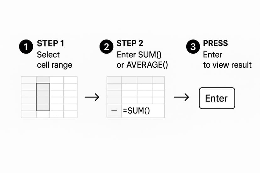
It’s a great reminder that even powerful formulas are often just a few clicks away.

Applying IF to a Business Scenario

Now, let's put this into a more practical business context. Say you're managing inventory and need to reorder any item that drops below 25 units in stock. Instead of manually scanning your list every day, you can get IF to do the work.

The formula would be: =IF(C2<25, "Reorder", "OK")

Here, the formula checks the stock level in cell C2. If it's less than 25, it flags the item with "Reorder." Otherwise, it displays "OK," letting you focus only on what needs attention.

This simple automation is a huge time-saver. You've just created a dynamic system that monitors your stock levels for you, replacing a tedious manual check.

Functions like IF are exactly why Excel has been an indispensable tool since 1985. They turn static data into something that can be analyzed and acted upon—a critical skill in finance, marketing, or any data-heavy role.

The IF function is a fantastic starting point for in-sheet automation. As you get more comfortable, you might also want to explore general approaches to automate repetitive tasks that can streamline your work even further. Mastering this one function is your gateway to building much smarter and more responsive spreadsheets.

Cleaning and Combining Text with Formulas

While Excel is a powerhouse for numbers, it's equally brilliant at manipulating text. If you've ever imported data from another program, you know the headache—it often arrives messy and inconsistent. This is where text formulas come to the rescue, saving you from hours of manual cleanup.

With just a few keystrokes, these simple Excel formulas for beginners can take a jumble of text and turn it into clean, usable data. Need to join a first and last name? Standardize capitalization? There’s a formula for that.

Joining Text with CONCAT

One of the most common text-related tasks is combining information from different cells. Let's say you have first names in one column and last names in another, but you need a single "Full Name" column. The CONCAT function is your go-to tool.

It does exactly what it sounds like: it concatenates, or joins, text strings together. So, if cell A2 contains "Jane" and B2 contains "Doe," the formula =CONCAT(A2, " ", B2) results in "Jane Doe." That " " in the middle is crucial—it adds the space. Without it, you'd end up with "JaneDoe."

Tidying Up with TRIM and Capitalization Functions

Messy data is a major obstacle. Extra spaces and inconsistent capitalization can throw off your other formulas, especially when trying to sort, filter, or look up information. Thankfully, Excel provides simple functions to instantly whip your text into shape.

TRIM: This function is a lifesaver. It removes all extra spaces from a cell, leaving just a single space between words. So if a cell reads " John Smith ", =TRIM(A1) cleans it up to a perfect "John Smith."
UPPER, LOWER, and PROPER: These three give you total control over case. UPPER makes everything uppercase (JANE DOE), LOWER makes it all lowercase (jane doe), and PROPER capitalizes the first letter of each word (Jane Doe). The PROPER function is particularly useful for names and titles.

Getting comfortable with functions like TRIM and PROPER is a key data cleaning skill. When your data is consistently formatted, it doesn't just look better; it's far more reliable for any analysis you do later, preventing errors in sorting, filtering, and charts.

You can even nest these formulas to perform multiple actions at once. For instance, =PROPER(TRIM(A1)) first strips out any unwanted spaces and then applies proper capitalization. It solves two common data problems in a single, elegant step.

While these formulas are fantastic for putting text together, sometimes you need to pull it apart. For that, check out our guide on how to split text in Excel—it's another essential skill for your data toolkit.

Dodging Common Beginner Pitfalls

Knowing the right formulas is half the battle; using them correctly is what truly saves time and prevents frustration. As you start out with Excel formulas for beginners, you're bound to run into a few common tripwires. Let's walk through how to spot and sidestep them from day one.

One of the most frequent mistakes is hard-coding numbers directly into a formula. Imagine calculating a 5% sales tax by writing =A2 * 0.05. It works, but what happens when the tax rate changes? You're stuck manually finding and updating every single formula.

Point to Cells, Don't Type in Numbers

Here’s a much smarter way to work. Put that tax rate (0.05) into its own dedicated cell, say F1. Then, your formula becomes =A2 * $F$1. That small change is a game-changer. If the rate ever changes, you update it in one spot, and every calculation that uses it updates instantly. This makes your spreadsheet flexible and far easier to manage.

Another pro tip is to use parentheses () to control the order of operations. Excel follows standard math rules (PEMDAS), but wrapping parts of your formula in parentheses removes any ambiguity. For example, = (A1+A2) / 2 (the average of two numbers) gives a totally different result than =A1 + A2/2 (A1 plus half of A2).

Forcing Excel to calculate parts of your formula in a specific order with parentheses is a fundamental best practice. It removes any doubt about how the final result is calculated, making your formulas both predictable and easier for others to understand.

Making Sense of Formula Errors

Sooner or later, you’ll see an error message like #NAME? or #DIV/0!. Don't panic! These are just Excel's signals telling you what went wrong. Learning to decode them is a crucial skill.

#NAME? This almost always means you've misspelled something. Check your function name—did you type AVRAGE instead of AVERAGE? It's an easy fix.
#DIV/0! This one’s clear: your formula is trying to divide by zero, which is mathematically impossible. This usually happens when a cell you're referencing is blank or contains a 0.
#REF! You'll get this error when a formula is pointing to a cell that no longer exists, likely because you deleted the row or column it was in.

Figuring out these issues is just part of the learning process. If you find yourself stuck, our guide on common Excel formula troubleshooting can help you dig deeper.

When you join the global user base of Excel, estimated to be between 1.1 billion and 1.5 billion people, you realize just how important these best practices are. With over 71,000 people in the U.S. alone using it for document management, building these good habits early will make your skills that much more valuable. You can discover more insights about Excel's widespread use on scottmax.com.

Got Questions About Excel Formulas? Let's Answer Them.

As you start getting comfortable with Excel formulas, a few questions always pop up. Let's tackle some of the most common ones beginners ask to help clear up any lingering confusion and get you working more confidently.

Think of this as the "aha!" section where the last few pieces of the puzzle click into place.

How Do I Copy a Formula Down a Column?

This is one of the best time-savers in Excel. Once you've written your formula in the first cell, just click on it.

See that small green square in the bottom-right corner? That's the fill handle. Hover your mouse over it until the cursor turns into a thin black plus sign. Then, just click and drag it all the way down the column. Excel cleverly copies the formula for you, automatically updating the cell references for each new row.

What's the Difference Between a Relative and an Absolute Reference?

Understanding this concept is a game-changer for building robust spreadsheets that don't break. It's simpler than it sounds.

Relative Reference (e.g., A1): This is Excel's default. When you copy a formula, the cell references adjust relative to their new location. If you copy a formula one cell down, its references also shift one cell down.
Absolute Reference (e.g., $A$1): The dollar signs lock the reference. No matter where you copy the formula, it will always point back to that specific cell.

A great way to think about it: use relative references for values that change with each row, like an item's price. Use an absolute reference for a single, constant value that applies to everything, like a fixed sales tax rate.

Actionable Tip: While typing a formula, you can press the F4 key on your keyboard to cycle through the different reference types ($A$1, A$1, $A1, A1). It's much faster than manually typing the dollar signs.

Can AI Help Me with Excel Formulas?

Absolutely. The rise of artificial intelligence has introduced powerful new ways to work with Excel, eliminating the need to memorize complex syntax. AI-powered tools act as your personal assistant, generating the exact formula you need based on a simple description of your goal.

For example, instead of trying to remember the VLOOKUP or INDEX/MATCH functions, you could simply ask an AI tool: "Find the price of the product in cell A2 from the price list on the 'Products' sheet." The AI would then generate the correct formula for you, saving time and preventing errors. This approach allows you to focus on the problem you're trying to solve rather than the technical details of the formula.

Ready to stop Googling formulas and start getting instant answers? Elyx.AI plugs right into Excel and lets you generate formulas, build pivot tables, and clean up your data just by asking in plain English. It's like having an expert sitting next to you. See how Elyx.AI can change the way you work in Excel.