7 Essential Excel Formula Examples for 2025

While almost everyone knows =SUM(), Excel's true power for business intelligence is unlocked through its more advanced functions. In a data-centric professional environment, mastering a core set of formulas is no longer a niche skill-it's a fundamental requirement for making smarter, faster business decisions. This guide moves beyond the basics to provide powerful, practical Excel formula examples that solve complex, real-world problems. We will dissect the syntax, strategic application, and common pitfalls for seven essential formulas that are critical for modern data analysis.

You will learn how to execute dynamic lookups with INDEX & MATCH, create sophisticated conditional summaries with SUMIFS and COUNTIFS, and implement logical decision-making with IF statements. This is not just a list of functions; it is a strategic breakdown of why these specific formulas are indispensable for tasks like financial modeling, sales performance reporting, and project management analytics. Each example provides actionable takeaways you can immediately apply. We will also enhance these examples with AI-powered tips from Elyx.AI, demonstrating how to automate and accelerate these tasks, transforming raw datasets into clear, decisive insights. Let's dive into the formulas that will elevate your data skills.

1. VLOOKUP – Vertical Lookup Formula

The VLOOKUP function is a cornerstone of data analysis in Excel, enabling users to search for a specific value in the first column of a data table and retrieve a corresponding value from another column in the same row. Its name stands for "Vertical Lookup," as it scans down a column to find your target. This function is indispensable for merging datasets, automating reports, and cross-referencing information without manual effort.

The formula syntax is =VLOOKUP(lookup_value, table_array, col_index_num, [range_lookup]). For instance, in an employee database, you could use it to find an employee's salary by searching for their unique Employee ID. It's one of the most fundamental excel formula examples for anyone in finance, operations, or data management.

Strategic Application: When and Why to Use VLOOKUP

VLOOKUP excels when you need to pull specific information from a large, structured table into another sheet or report. It's the go-to function for tasks like:

• Pricing Lookups: Retrieving the price of a product from a master catalog based on its SKU.
• Contact Information: Pulling a customer's phone number or address from a CRM export using their name or ID.
• Inventory Checks: Finding the current stock level for a specific item in an inventory list.

The key is that your lookup value must be in the leftmost column of your data source. This limitation is crucial to remember when structuring your data for analysis.

Deciding on Your Lookup Strategy

Choosing the right lookup approach is critical for data integrity. The following decision tree visualizes a simple thought process for selecting the correct lookup function based on your specific needs, focusing on VLOOKUP's capabilities versus more flexible alternatives like INDEX and MATCH.

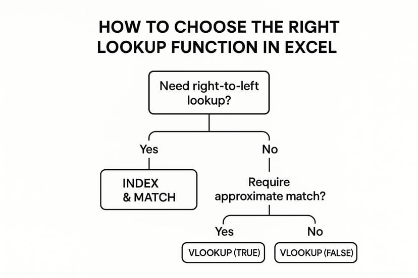
This flowchart clarifies that while VLOOKUP is powerful, it's best used for standard, left-to-right lookups where you can specify whether you need an exact or an approximate match.

Actionable Takeaways & Best Practices

To master VLOOKUP, apply these tactical insights to ensure accuracy and efficiency in your spreadsheets.

Key Strategy: Always set the range_lookup argument to FALSE for an exact match in business applications. This prevents Excel from returning an incorrect, approximate match, which can lead to significant reporting errors.

• Stabilize Your Table Array: When copying your formula down a column, use absolute references for the table_array (e.g., $A$2:$D$100). This locks the reference and prevents it from shifting.
• Handle Errors Gracefully: Wrap your VLOOKUP formula within an IFERROR function (e.g., =IFERROR(VLOOKUP(...), "Not Found")). This replaces ugly #N/A errors with a clean, custom message.
• Use Named Ranges: For improved readability and easier management, define your table_array as a named range (e.g., "ProductCatalog") instead of using cell references.

2. INDEX and MATCH – Dynamic Lookup Combination

The combination of INDEX and MATCH is a powerful, flexible lookup method that overcomes the primary limitations of VLOOKUP. INDEX retrieves a value from a specific row and column within a range, while MATCH finds the position of a lookup value in a row or column. When used together, they create a superior lookup system that can pull data from any column, regardless of its position relative to the lookup column.

The combined syntax is =INDEX(return_array, MATCH(lookup_value, lookup_array, 0)). For example, in an HR database, you could find an employee's start date (Column A) by searching for their name (Column D), something VLOOKUP cannot do. This dynamic duo is one of the most essential excel formula examples for analysts who need robust and adaptable data retrieval solutions.

Strategic Application: When and Why to Use INDEX and MATCH

INDEX and MATCH shine in scenarios where data is not perfectly structured for a simple VLOOKUP. It's the ideal choice when you need a more resilient and versatile lookup. Use it for:

• Leftward Lookups: Finding data in columns to the left of your lookup column, like retrieving an Employee ID using a name.
• Dynamic Column Selection: Allowing users to select which column's data to return (e.g., from a dropdown menu), making reports interactive.
• Stable References: Creating formulas that don't break when new columns are inserted or deleted from the source data table.
• Horizontal and Vertical Lookups: Performing lookups both vertically (down a column) and horizontally (across a row) with minor formula adjustments.

Its key advantage is decoupling the lookup column from the return column, providing unparalleled flexibility in spreadsheet design and data analysis.

Deciding on Your Lookup Strategy

Choosing between VLOOKUP and INDEX/MATCH depends entirely on your data structure and future needs. If you need a lookup that can search in any direction and is immune to changes in table structure, INDEX/MATCH is the superior professional choice.

This combination works by first using MATCH to find the row number of your lookup value. Then, INDEX takes that row number and retrieves the corresponding value from the separate return column you specified. This two-step process makes it more robust than VLOOKUP's rigid, all-in-one approach. While the new XLOOKUP function now handles many of these cases, understanding INDEX/MATCH is crucial for working in older versions of Excel and for mastering advanced spreadsheet logic.

Actionable Takeaways & Best Practices

To effectively implement INDEX and MATCH, focus on building the formula logically and ensuring each part functions correctly.

Key Strategy: Always use 0 as the third argument in the MATCH function for an exact match. This is the equivalent of VLOOKUP's FALSE and is critical for preventing incorrect results in most business contexts.

• Build and Test Separately: First, write your MATCH function in a separate cell to ensure it correctly returns the row number you expect. Then, build the INDEX function around it.
• Use Full Column References: For simpler formulas and to accommodate growing datasets, use full column references like A:A for the return_array and C:C for the lookup_array. Be aware this can slow down very large workbooks.
• Combine with IFERROR: Just like VLOOKUP, wrap your INDEX/MATCH formula in an IFERROR function (e.g., =IFERROR(INDEX(...), "Data Not Available")) to manage #N/A errors cleanly.
• Leverage Named Ranges: Define your lookup and return arrays with named ranges (e.g., "EmployeeNames", "SalaryData") to make your formulas self-documenting and much easier to read and audit.

3. SUMIF and SUMIFS – Conditional Sum Formulas

The SUMIF and SUMIFS functions are powerful tools for summarizing data based on specific conditions. SUMIF adds up values in a range that meet a single criterion, while its more versatile counterpart, SUMIFS, can handle multiple criteria across different ranges. This capability allows you to move from raw data to insightful summaries with a single formula, making them essential excel formula examples for anyone performing targeted data analysis.

The syntax for SUMIF is =SUMIF(range, criteria, [sum_range]), and for SUMIFS, it's =SUMIFS(sum_range, criteria_range1, criteria1, ...). For example, you could use SUMIF to calculate total sales for a single region or SUMIFS to find total sales for a specific product within that region during a particular quarter.

Strategic Application: When and Why to Use Conditional Sums

SUMIF and SUMIFS are indispensable when you need to aggregate data conditionally without creating pivot tables or manually filtering. They are perfect for building dynamic dashboards and reports. Use them for:

• Sales Reporting: Calculating total revenue by region, product, or specific salesperson.
• Budget Analysis: Summing expenses by department and category to track spending against targets.
• Inventory Management: Valuing stock by location, category, or supplier to understand where your assets are.
• Performance Metrics: Aggregating employee commission totals based on multiple performance tiers.

These functions shine when you need to answer specific business questions directly from a large dataset, turning complex tables into clear, actionable numbers. To explore more advanced techniques, you can learn more about data transformation in Excel.

Deciding on Your Summation Strategy

Choosing between SUMIF and SUMIFS depends entirely on the complexity of your question. SUMIF is quick and effective for one-condition summaries, like "total sales in the North region." However, when your query involves multiple constraints, such as "total sales of 'Product A' in the 'North' region for 'Q1'," SUMIFS is the necessary and more robust tool. Always lean towards SUMIFS if you anticipate needing to add more criteria later, as it is more scalable.

Actionable Takeaways & Best Practices

To leverage conditional sums effectively, focus on precision and scalability. These tips will help you build reliable and error-free formulas.

Key Strategy: Always use quotation marks for text criteria (e.g., "North") and when using logical operators with numbers (e.g., ">1000"). This ensures Excel correctly interprets your conditions.

• Concatenate for Flexibility: Use the ampersand (&) to combine operators with cell references (e.g., ">"&B1). This allows you to create dynamic criteria that update when the referenced cell changes.
• Use Excel Tables: Format your data source as an Excel Table. This allows you to use structured references (e.g., TableName[ColumnName]), which automatically expand as you add new data, keeping your formulas up-to-date.
• Ensure Range Consistency: In SUMIFS, make sure all criteria_range arguments have the exact same number of rows and columns as the sum_range to avoid a #VALUE! error.

4. IF Statement – Logical Decision Making

The IF function is the core of logical decision-making in Excel, allowing your spreadsheets to react dynamically to your data. It evaluates a condition you set and returns one value if that condition is true and another if it's false. This function is fundamental for creating models, dashboards, and reports that automatically update based on changing inputs, moving beyond static calculations.

The formula syntax is =IF(logical_test, value_if_true, value_if_false). For instance, in a sales report, you could use it to label a salesperson as "Bonus Eligible" if their sales exceed a target. The IF statement is one of the most essential excel formula examples for anyone needing to automate decisions and create responsive analytical tools.

Strategic Application: When and Why to Use IF

The IF statement excels in any scenario where you need to apply business rules or conditional logic directly within your worksheet. It is the ideal function for tasks like:

• Project Status Tracking: Automatically displaying "On Track," "Delayed," or "At Risk" based on deadline proximity.
• Budget Variance Analysis: Flagging line items as "Over Budget" if actual spending exceeds the planned amount.
• Inventory Management: Labeling items as "Reorder" when stock levels fall below a specific threshold.
• Grade Calculation: Assigning pass/fail status to students based on their scores.

The function’s power lies in its simplicity for binary outcomes. For more complex, multi-tiered logic, you can nest IFs or use the more modern IFS function.

Deciding on Your Logical Strategy

Choosing the correct logical function is crucial for building clean, efficient, and error-free formulas. For simple true/false tests, the standard IF function is perfect. However, when your logic involves multiple conditions, you must decide whether to nest multiple IF statements or use newer, more streamlined functions like IFS or SWITCH. For robust data entry, you can combine IF logic with data validation rules. For more details on this, you can learn more about how to set up powerful data validation on getelyxai.com. This approach ensures both calculation accuracy and data integrity from the start.

Actionable Takeaways & Best Practices

To leverage the IF function effectively, apply these tactical insights to make your formulas more powerful, readable, and manageable.

Key Strategy: For multiple conditions, use the IFS function (=IFS(test1, value1, test2, value2, ...)). It eliminates the need for complex, deeply nested IF statements, making your formulas easier to write, audit, and debug.

• Combine with AND/OR: For compound logical tests, embed AND or OR functions inside your logical_test (e.g., =IF(AND(A2>10, B2<50), "Pass", "Fail")).
• Plan Your Logic: Before writing a complex formula, map out the conditions and outcomes on paper or in comments. This prevents logical errors and simplifies the construction process.
• Return Blanks for Clarity: To keep your sheet clean, you can return an empty string ("") instead of a 0 or FALSE (e.g., =IF(A2>0, A2, "")).

5. CONCATENATE and TEXTJOIN – Text Combination Functions

Manipulating text is just as important as crunching numbers, and Excel provides powerful functions for this purpose. The CONCATENATE function and its more modern successor, TEXTJOIN, are essential for combining text from multiple cells into a single, cohesive string. While CONCATENATE simply merges text strings one by one, TEXTJOIN offers greater flexibility by allowing a delimiter and the option to ignore empty cells.

The syntax for CONCATENATE is =CONCATENATE(text1, [text2], ...), while TEXTJOIN is =TEXTJOIN(delimiter, ignore_empty, text1, [text2], ...). These are fundamental excel formula examples for anyone who needs to clean data, format reports, or generate dynamic labels from disparate pieces of information.

Strategic Application: When and Why to Use Text Combination

These functions are invaluable when you need to assemble meaningful information from raw, fragmented data. They are the go-to solution for tasks like:

• Full Name Creation: Combining separate "First Name" and "Last Name" columns into a single "Full Name" field.
• Address Formatting: Assembling a complete mailing address from individual components like street, city, state, and zip code.
• Product Code Generation: Creating unique product identifiers by merging attributes like category, size, and color codes.
• Dynamic Report Titles: Generating descriptive titles for reports, such as "Sales Summary for " followed by a dynamic date.

CONCATENATE (or the simpler & operator) works for basic joins, but TEXTJOIN is superior when dealing with ranges or needing consistent separators.

Deciding on Your Combination Strategy

Choosing the right text combination method depends on the complexity of your task. For joining just two or three cells, the ampersand (&) operator is often the quickest. For combining a whole range of cells with a consistent separator like a comma, TEXTJOIN is vastly more efficient and cleaner than a nested CONCATENATE formula.

For example, creating a comma-separated list of team members from a range A2:A10 is simple with TEXTJOIN (=TEXTJOIN(", ", TRUE, A2:A10)) but would be incredibly tedious with CONCATENATE. This decision-making process ensures your formulas are both effective and easy to maintain.

Actionable Takeaways & Best Practices

To become proficient at combining text, use these tactical insights to produce clean, well-formatted data.

Key Strategy: Default to using TEXTJOIN over CONCATENATE in modern versions of Excel (2019 and later). Its ability to handle delimiters and ignore empty cells across a range makes formulas shorter, more readable, and less prone to error.

• Use the & Operator for Simplicity: For quick, one-off combinations like =A2&" "&B2 to join a first and last name, the & operator is often the most direct method.
• Handle Line Breaks: To create multi-line text within a single cell, use CHAR(10) as your delimiter in TEXTJOIN (e.g., =TEXTJOIN(CHAR(10), TRUE, A2:D2)). Remember to enable "Wrap Text" for the cell.
• Clean Your Data First: Wrap your source cell references within the TRIM function (e.g., TRIM(A2)) before concatenating to remove any leading or trailing spaces that could cause formatting issues.
• Include Necessary Punctuation: Remember to add spaces or punctuation as part of your text strings or delimiters, such as ", " in TEXTJOIN or " " in CONCATENATE, to ensure the final output is readable.

6. COUNTIF and COUNTIFS – Conditional Counting Functions

The COUNTIF and COUNTIFS functions are essential for data summarization, allowing you to count the number of cells within a range that meet specific conditions. COUNTIF handles a single criterion, while COUNTIFS extends this capability to evaluate multiple criteria across different ranges simultaneously. This makes them indispensable tools for creating dashboards, tracking metrics, and performing quick data audits.

The syntax for COUNTIF is =COUNTIF(range, criteria), and for COUNTIFS, it is =COUNTIFS(criteria_range1, criteria1, [criteria_range2, criteria2], ...). For instance, you could count how many sales transactions exceeded $500 from a specific region. These functions are some of the most practical excel formula examples for anyone needing to distill large datasets into meaningful numbers.

Strategic Application: When and Why to Use COUNTIF/COUNTIFS

COUNTIF and COUNTIFS are your go-to functions when you need to answer "how many" based on specific conditions. They are perfect for turning raw data into quantitative insights without complex filtering or PivotTables. Use them for tasks like:

• Sales Performance: Counting the number of deals closed by a specific salesperson that are over a certain value.
• Inventory Management: Identifying how many products in an inventory list are below their reorder level.
• Survey Analysis: Tallying responses to a survey question, such as counting how many respondents selected "Strongly Agree."
• Quality Control: Tracking the number of products that failed inspection based on a "Fail" status in a log.

These functions shine when you need a quick, dynamic count that updates as your source data changes, providing real-time summaries directly in your worksheet.

Deciding on Your Counting Strategy

Choosing between COUNTIF and COUNTIFS depends entirely on the complexity of your question. If you are evaluating just one condition, such as "how many tasks are marked 'Complete'?", COUNTIF is sufficient and simpler. However, if your query involves multiple conditions, like "how many 'High Priority' tasks are 'Overdue'?", you must use COUNTIFS.

This distinction is crucial for accurate data analysis. Using COUNTIF for a multi-conditional query would require cumbersome nested formulas or helper columns, whereas COUNTIFS handles it elegantly in a single, readable formula.

Actionable Takeaways & Best Practices

To leverage conditional counting effectively, apply these tactical insights to build robust and error-free reports.

Key Strategy: Use wildcards for flexible text matching. The asterisk * represents any sequence of characters, while the question mark ? represents any single character. For example, COUNTIF(A:A, "Apple*") would count cells containing "Apple," "Apples," or "Apple Inc."

• Combine with Comparison Operators: Enclose numeric criteria with operators in double quotes (e.g., ">500", "<>"&B2). This allows you to count cells that are greater than, less than, or not equal to a specific value or cell reference.
• Ensure Range Consistency: When using COUNTIFS, make sure all your criteria_range arguments have the exact same number of rows and columns. Mismatched ranges will result in a #VALUE! error.
• Count Non-Blanks and Blanks: For a simple tally of all non-empty cells, use COUNTA(range). To count only empty cells, use COUNTBLANK(range). These are often faster alternatives for basic presence checks.

7. PIVOT TABLE Formulas – Advanced Data Summarization

While not a single function, PivotTable formulas represent a powerful suite of tools for dynamic data summarization and analysis. At its core, a PivotTable is an interactive report that allows you to quickly aggregate, filter, and cross-tabulate large datasets without writing complex formulas. The key formula associated with this feature is GETPIVOTDATA, which retrieves specific data points from a completed PivotTable report.

The syntax for this function is =GETPIVOTDATA(data_field, pivot_table, [field1, item1], ...). For example, you could use it to pull the total sales figure for "Laptops" in the "North" region directly into a separate summary dashboard. This combination of interactive reporting and targeted data extraction makes PivotTables one of the most essential excel formula examples for transforming raw data into business intelligence.

Strategic Application: When and Why to Use PivotTables

PivotTables are unparalleled when you need to explore and summarize multidimensional data interactively. They are the ideal solution for building reports that require slicing and dicing information from different perspectives. Key use cases include:

• Sales Dashboards: Analyzing sales performance by region, product, and salesperson.
• Financial Reporting: Creating dynamic income statements or budget variance reports.
• HR Analytics: Summarizing workforce data by department, tenure, and performance rating.
• Operations Metrics: Tracking production efficiency by shift, machine, and product line.

The primary advantage is the ability to drag and drop fields to instantly reconfigure your report, allowing for rapid exploration and insight generation without rebuilding formulas. For a deeper dive, you can explore our guide on creating PivotTables in Excel.

Actionable Takeaways & Best Practices

To leverage the full power of PivotTables, apply these tactical insights for robust and efficient data analysis.

Key Strategy: Use Calculated Fields to create custom metrics directly within your PivotTable. This avoids adding extra columns to your source data and keeps your analysis self-contained and easy to update.

• Clean Source Data: Ensure your source data is in a proper tabular format with no blank rows or columns before creating a PivotTable. This is the single most important step for accuracy.
• Refresh Your Data: PivotTables do not update automatically when the source data changes. Always right-click and select "Refresh" to ensure your report reflects the latest information.
• Control GETPIVOTDATA: By default, Excel generates GETPIVOTDATA formulas when you reference a cell in a PivotTable. You can disable this feature via the "PivotTable Analyze" tab if you prefer standard cell references.
• Visualize with PivotCharts: Connect a PivotChart to your PivotTable to create a dynamic visual representation of your summary data that updates automatically as you filter or change the table layout.

7 Key Excel Formula Examples Comparison

Function / Feature	Implementation Complexity 🔄	Resource Requirements ⚡	Expected Outcomes 📊	Ideal Use Cases 💡	Key Advantages ⭐
VLOOKUP – Vertical Lookup	Low; simple syntax, single function	Low; works efficiently on large data	Fast exact/approximate lookups vertically	Database lookups, pricing, inventory, CRM	Easy to learn; widely supported; fast on large sets
INDEX and MATCH	Medium-High; combines two functions	Moderate; robust with large datasets	Flexible bi-directional lookups	Complex reports, dynamic models, multi-column searches	Flexible; handles left lookups; robust to structure changes
SUMIF and SUMIFS	Low; straightforward condition syntax	Low; efficient with large datasets	Conditional summation with 1+ criteria	Sales reports, budgeting, inventory, commissions	Eliminates helper columns; supports multiple criteria
IF Statement	Low-Medium; basic logic but nesting adds complexity	Low; minimal resource use	Logical branching and decision making	Grade calculations, commissions, status tracking	Intuitive logic; versatile; essential for dynamic formulas
CONCATENATE and TEXTJOIN	Low; simple text joining functions	Low; efficient for text operations	Combined text outputs with delimiters	Names, addresses, codes, signatures	Flexible delimiters; handles ranges (TEXTJOIN); cleaner output
COUNTIF and COUNTIFS	Low; similar to SUMIF but counts	Low; fast processing large data	Conditional counts with 1+ criteria	Surveys, quality control, sales metrics	Intuitive syntax; fast; supports complex criteria
PIVOT TABLE Formulas	High; requires data structuring and deeper understanding	Moderate to High; handles very large data	Dynamic summaries and drill-down analysis	Executive reporting, dashboards, multi-dimensional analysis	Powerful summarization; no formulas needed for basics

From Formulas to Fluent Insights: Your Next Step in Excel Mastery

We've journeyed through a powerful collection of seven essential Excel formula examples, moving from fundamental lookups to dynamic, multi-conditional data aggregation. The path from VLOOKUP to PIVOT TABLE formulas isn't just about memorizing syntax; it's about fundamentally changing how you interact with data. By mastering these functions, you transform your spreadsheets from static repositories of information into dynamic engines for analysis and decision-making.

The core principle unifying these examples is the strategic application of logic. Whether you're choosing between the straightforward VLOOKUP and the more flexible INDEX and MATCH combination, or layering conditions with SUMIFS and COUNTIFS, the goal remains the same: to ask sophisticated questions of your data and receive precise, actionable answers.

Key Takeaways for Advanced Spreadsheet Analysis

The strategic insights from these formulas empower you to build more resilient, efficient, and insightful workbooks. Remember these critical takeaways as you apply what you've learned:

• Prioritize Flexibility: While VLOOKUP is a reliable workhorse, the INDEX and MATCH combination offers superior flexibility, allowing lookups in any direction and preventing errors when columns are inserted or deleted. This adaptability is a hallmark of advanced spreadsheet design.
• Embrace Conditional Logic: Functions like IF, SUMIFS, and COUNTIFS are the building blocks of intelligent analysis. They allow you to segment, filter, and calculate based on specific criteria, turning raw data into meaningful business intelligence.
• Structure for Clarity: The power of TEXTJOIN over the classic CONCATENATE highlights a key theme: modern Excel functions are designed for efficiency and cleaner formulas. Always choose the tool that makes your work more readable and easier to debug.

A well-structured formula is more than just functional; it's a piece of documentation. Your future self, and your colleagues, will thank you for prioritizing clarity and resilience in your workbook architecture.

Your Path from Manual Formulas to Automated Insights

Mastering these seven Excel formula examples provides an incredible foundation. You now possess the toolkit to tackle complex challenges in financial modeling, project management, and operational reporting. The next step in your journey is not just learning more formulas, but accelerating how you build and deploy them. This is where the strategic advantage of AI comes into play.

The transition from manual formula construction to AI-assisted analysis represents a significant leap in productivity. Instead of spending valuable time troubleshooting a complex nested IF statement or searching for the correct syntax, you can leverage tools that understand your analytical intent. This frees you up to focus on higher-level strategic questions, interpreting the results and driving business outcomes rather than getting bogged down in the mechanics. The future of data analysis is collaborative, with human expertise guided and amplified by artificial intelligence.

---

Ready to supercharge your spreadsheet workflow and generate complex formulas with simple text commands? Explore how Elyx.AI can become your personal Excel co-pilot, automating tedious tasks and unlocking deeper insights in seconds. Visit Elyx.AI to see how you can move beyond manual formula creation and into the future of data analysis.