Excel Formula Troubleshooting Your Ultimate Guide

We’ve all been there. You spend time crafting what you think is the perfect Excel formula, hit Enter, and… nothing. Instead of the neat, calculated result you expected, the formula text itself just sits there, mocking you. It’s one of the most common frustrations in Excel, but the good news is that it’s almost always a quick fix.

Usually, this problem boils down to one of two simple things: either your cell is formatted incorrectly, or you've accidentally switched Excel into a special viewing mode. Let's walk through how to spot and solve these in seconds.

The Cell Is Formatted as Text

This is the number one reason I see formulas failing to calculate. If a cell is formatted as Text, Excel takes you literally. It sees =SUM(A1:A5) and thinks you just want to display that exact text string, not perform a calculation. It won't even try to run the formula.

The fix is easy. Just select the problematic cell (or cells), go to the Home tab, and in the "Number" group, change the format from Text to General.

Here's the crucial final step: Changing the format isn't enough. You have to "re-enter" the formula to make Excel re-evaluate it. The quickest way is to select the cell, press F2, and then immediately press Enter. The formula will spring to life.

You've Accidentally Flipped on "Show Formulas" Mode

Ever hit a random keyboard shortcut and suddenly your entire spreadsheet looks broken? You might have stumbled into "Show Formulas" mode. It’s a genuinely useful feature for auditing your work, as it displays all the formulas on a sheet instead of their results. If you don’t know it’s on, however, it just looks like everything stopped working.

This mode is a simple toggle. One key combination turns it on, and the same one turns it off.

Take a look at the screenshot—see how cell B5 shows the SUM function text instead of the actual total, 150? That’s "Show Formulas" in action.

To get your results back, just press **Ctrl + ** (that's the backtick key, usually located to the left of the 1` key). Your sheet will instantly return to normal.

For a deeper dive, our guide on real-world Excel formula examples can give you more hands-on practice to build your confidence and avoid these common roadblocks.

We’ve all been there: staring at a #N/A or #VALUE! error, randomly tweaking parts of a formula, and hoping for the best. That approach is a fast track to frustration. The real trick is to stop guessing and start investigating. Think of yourself as a formula detective, using a structured approach to pinpoint exactly where things went wrong.

Excel actually gives you some fantastic, built-in auditing tools for this very purpose. When you learn how to use them, you move from just fixing the immediate problem to understanding the why behind it. This not only solves your current headache but also makes you a much more confident and capable Excel user down the road.

This simple visual breaks down the core process for tackling any formula error you encounter.

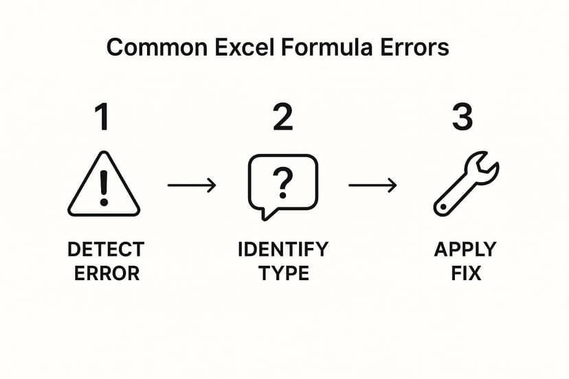
It boils down to a three-part mental model: spot the error, figure out what kind of error it is, and then apply the right solution. It’s a reliable framework for any troubleshooting scenario.

Follow the Data Trail with Trace Precedents

One of the best tools in your detective kit is Trace Precedents. You can find it in the "Formulas" tab, and it's a lifesaver. When you select a cell with a formula and click this button, Excel draws arrows showing you every single cell that feeds data into your calculation. It’s like creating a visual map of your formula's DNA.

Let's say you have a complex SUMIFS in a sales report that's giving you the wrong total. Instead of manually double-checking every cell range, just click Trace Precedents. Blue arrows will instantly point out the exact ranges being used for the sum and the criteria. More often than not, you'll see the problem right away—a range that's off by one row or a criteria that's pointing to the wrong column. It’s especially powerful when you’re trying to make sense of a spreadsheet someone else built.

Go Step-By-Step with Evaluate Formula

Sometimes, just seeing the input cells isn't enough. You need to see how Excel is thinking. That’s where the Evaluate Formula tool comes in. This feature is like a slow-motion replay of your formula's logic. It opens a small window and lets you "evaluate" your formula one piece at a time.

Imagine a nested formula like =IF(VLOOKUP(A2, SalesData, 2, FALSE)>5000, "High", "Low"). It has a few moving parts. Using Evaluate Formula, you can see what the VLOOKUP part resolves to first. Does it find a value, or does it return an error?

Pro Tip: Each time you click the "Evaluate" button, Excel shows you the calculated value for the underlined part of the formula. This lets you watch the calculation unfold. You can see the exact moment a VLOOKUP returns an error or when the comparison to 5000 gives you an unexpected TRUE or FALSE.

This methodical breakdown turns a big, confusing formula into a series of small, easy-to-check steps. This is the heart of effective Excel formula troubleshooting—transforming a tangled mess into a solvable puzzle.

Decoding Common Excel Error Messages

We’ve all been there. You’re deep in a spreadsheet, and suddenly a cell screams #DIV/0!, #VALUE!, or #NAME? back at you. It’s easy to get frustrated, but these aren't just dead ends. They're actually clues Excel gives you, pointing right to the problem.

Learning to read these messages is a fundamental skill in Excel formula troubleshooting. Instead of seeing a broken formula, you start to see a clear path to a fix. Think of it as Excel’s way of trying to help. So, let's break down what these common errors are really telling you.

The Infamous #DIV/0! Error

This is probably the first error most of us ever run into. It’s straight-up math—you can't divide a number by zero. In the real world, I see this all the time in financial models or inventory trackers where a cell in the denominator is empty or has a zero value.

Imagine you're tracking Cost Per Unit with a simple =TotalCost / UnitsSold formula. For any brand-new products, UnitsSold is likely zero, which immediately throws the #DIV/0! error. You could go in and manually change the data, but that's not a scalable solution. A much better approach is to anticipate the error.

This is where the IFERROR function becomes your best friend.

Wrap your original calculation in IFERROR. For example: =IFERROR(TotalCost / UnitsSold, "Not Calculated"). Now, instead of a jarring error, your spreadsheet displays clean, custom text. It makes your reports look far more professional.

The Mysterious #### Error

Seeing a cell filled with hash marks (####) looks alarming, but the fix is almost always incredibly simple. This isn't a formula error at all; it's a formatting issue. All it means is that your column isn't wide enough to display the full number or date inside the cell.

You’ll see this constantly with long date formats or large numbers. The quickest fix? Just find the right-hand border of the column header in question and double-click it. Excel will automatically resize the column to fit the widest entry. Simple as that. The #DIV/0! error is a frequent issue when a formula attempts to divide by zero, while the #### error typically indicates that a column is too narrow to display its contents. Dive into more Excel error solutions to sharpen your skills.

Understanding #NAME? and #VALUE!

These two errors can seem similar, but they point to completely different problems. Getting them straight is key to fixing your formulas quickly.

The #NAME? Error: This error pops up when Excel doesn't recognize something you've typed into a formula. 99% of the time, it’s a typo in a function name, like VLOOKP instead of VLOOKUP. It can also happen if you reference a named range that you misspelled or that doesn't exist anymore.
The #VALUE! Error: This one is a bit broader and signals a data mismatch. It means you’re trying to perform an operation with the wrong type of argument. For example, if you try to do math with text, like =5 + "Apples", Excel will return a #VALUE! error. It's essentially saying, "I'm a calculator, and you just handed me a piece of fruit."

When you're stuck, Excel’s own Error Checking tool can be a huge help. It not only identifies the error but often explains the problem and suggests a fix, which can get you back on track without having to guess.

Tackling Problems with Advanced Tools Like Data Tables

As you get more comfortable in Excel, you'll naturally start using its more powerful analytical features, and Data Tables are a big one. They're fantastic for what-if scenarios, like figuring out how different interest rates and loan terms might change a monthly payment. But with this added power comes a whole new class of headaches when things go wrong.

Honestly, the most common mistake I see with Data Tables—and one I've made myself plenty of times—is a simple setup error. When you're building a two-variable table, Excel needs to know which cell is your "Row input" and which is your "Column input." It is ridiculously easy to get these backward. When you do, you're left with a table full of garbage values or just the same number repeated over and over, which is incredibly frustrating.

The Same-Sheet Rule: An Unbreakable Commandment

Here’s another rule that catches even veteran Excel users off guard: a Data Table must be on the same worksheet as its input cells. You simply can't point it to input cells on another tab. If you try, the table just won't calculate, and often you won't even get a clear error message telling you what's wrong.

This is a huge deal in complex financial models where your data is typically organized across many different sheets. The workaround is simple but crucial: just create direct cell links on your Data Table sheet that pull the values from the other tabs.

For instance, if your main interest rate input is sitting in cell B5 on a sheet named 'Summary', you’d go to your 'Analysis' sheet, pick a spare cell, and enter the formula ='Summary'!B5. Then, you use that new cell as the input for your Data Table. Problem solved.

The structure of a Data Table is rigid. The two most common reasons they break are mixing up the row and column inputs or trying to reference data on another sheet. Always check these two things first—it will save you a ton of time.

A Quick Sanity Check for Broken Data Tables

When your Data Table gives you nonsense, don't immediately tear it down and start over. Just run through this quick mental checklist. More often than not, the problem is right here.

Input Cells: Are you positive you picked the correct row and column input cells in the setup dialog? Double-check them.
Sheet Location: Are the input cells the table needs physically located on the same worksheet as the table itself?
Formula Link: Is the top-left corner cell of your Data Table grid pointing directly to the final output formula you want to analyze?
Calculation Setting: Is your workbook set to Automatic Calculation? If it's on manual, your table will never update until you force a recalculation (F9).

These advanced tools do follow strict, predictable rules. Once you learn their quirks, like the common input cell mix-up, you can spot the problem in seconds. Another frequent issue is misaligned input cells, which you can avoid by carefully verifying your row and column assignments. For a deeper dive into this specific problem, there are great tutorials on how to properly troubleshoot Data Tables.

Getting these checks down means you can confidently use Data Tables for some serious analysis. And if you're looking to boost your efficiency even more, it's worth learning how to automate Excel to minimize these kinds of manual errors from the very beginning.

How AI Can Supercharge Your Formula Troubleshooting

We’ve all been there. You've tried Excel's built-in tools, traced precedents, evaluated the formula step-by-step, and you're still staring at a stubborn #N/A or #VALUE! error. It's frustrating, especially when you're on a deadline. When you've hit that wall, AI tools can be your saving grace. This isn't about handing over the keys; it's about getting an expert co-pilot.

Think of a tool like Elyx.AI as having a formula wizard on call, 24/7. Instead of digging through old forum posts, you can just paste your broken formula into a chat and ask, "What's wrong with this?" The real magic is that it doesn’t just spit out a corrected version. It explains why it was broken in simple terms, which is invaluable for helping you learn and not make the same mistake twice.

Generate Perfect Formulas from Plain English

One of the best ways to fix errors is to prevent them from happening in the first place. This is where AI really shines. You can just describe what you want to do in plain English, and the AI handles the tricky syntax. This is a massive time-saver for notoriously complex functions, like nested IF statements.

Let's say you're building a sales commission calculator with a few performance tiers:

Below $10,000: 5% commission
$10,000 to $20,000: 7.5% commission
Over $20,000: 10% commission

Writing that nested IF by hand is a classic recipe for misplaced commas and parentheses. With a tool like Elyx.AI, you can just ask: "Create a formula that gives 5% commission for sales under 10000, 7.5% for sales between 10000 and 20000, and 10% for sales over 20000, based on cell C2."

Almost instantly, you get the clean, correct formula: =IF(C2>20000, C2*0.1, IF(C2>=10000, C2*0.075, C2*0.05))

By turning your plain-language goals directly into Excel's language, AI cuts out the human error that often creeps in when you're building complicated formulas. This not only saves a ton of time but also boosts your accuracy, which is critical for financial models or large datasets.

This capability is a game-changer when you're putting together complex reports. If you want to see how to take these AI-driven insights to the next level, our complete Excel dashboard tutorial is a great place to start visualizing your now error-free data.

More Than Just a Fixer-Upper

Using AI in Excel is about so much more than fixing what's broken. It fundamentally changes how you work. You get to spend more time thinking about the "what" and "why" of your analysis and less time getting bogged down in the technical weeds of formula syntax. It’s a way to genuinely boost your productivity and take on more ambitious projects with the confidence that you've got an intelligent assistant ready to back you up.

Your Top Excel Formula Questions, Answered

Even the most seasoned Excel pros get stumped by a formula that just won't cooperate. When you're staring down a deadline, a stubborn error can feel like a major roadblock. Let's tackle some of the most common questions that come up when you're wrestling with formulas, so you can get things working and move on.

Think of this as your go-to cheat sheet for those head-scratching "Why won't this work?!" moments.

Why Does My Cell Show the Formula Itself, Not the Answer?

This is a classic, and the solution is usually simple. When your formula appears as plain text instead of a calculated result, it’s almost always one of two things.

First, check the cell's formatting. If a cell is accidentally formatted as Text, Excel takes you at your word and displays the formula as a literal text string. To fix it, select the cell, head to the Home tab, and in the "Number" group, switch the format back to General. Here's the key part: you have to wake Excel up and make it re-evaluate. The easiest way is to click into the formula bar (or press F2) and then just hit Enter.

The other likely culprit is that you've unintentionally switched on "Show Formulas" mode. It's a handy feature for checking your work, but a real pain if you hit the shortcut by mistake.

A quick keyboard shortcut, Ctrl + ` (that's the backtick key, usually hanging out next to the 1 key), toggles this view. Press it, and your sheet should snap back to showing the results instead of the underlying formulas.

How Do I Get Rid of the #NAME? Error?

Seeing #NAME? is Excel’s polite way of telling you, "I have no idea what you're talking about." It means something in your formula isn't a recognized function, name, or text string.

Here’s where to look for the problem:

A typo in a function name: This happens to everyone and is the cause 99% of the time. It's so easy to type VLOOKP instead of VLOOKUP or SUMIF when you meant SUMIFS. A quick proofread is your first step.
A named range that doesn't exist: If your formula uses a named range, like =SUM(SalesTotal), you need to be sure that name has been created and spelled correctly. You can double-check all your existing named ranges by going to the Formulas tab and clicking on Name Manager.
Text strings without quotes: When you use text in a function, it needs to be wrapped in double quotes. A formula like =IF(A1=Active, "Yes", "No") will fail because Excel thinks "Active" is a function or named range. The fix is to put it in quotes: =IF(A1="Active", "Yes", "No").

What's the Best Way to Stop Errors Before They Start?

The best defense is a good offense. Instead of cleaning up a spreadsheet littered with ugly error codes, you can build in a safety net from the start. The most powerful tool for this is the IFERROR function.

Let's say you have a simple calculation, =A2/B2. This works fine until cell B2 is empty or contains a zero, at which point you get a glaring #DIV/0! error.

Wrapping your formula with IFERROR solves this beautifully. You'd write it as =IFERROR(A2/B2, 0) or perhaps =IFERROR(A2/B2, "N/A").

This instructs Excel to first attempt the A2/B2 calculation. If it works, great—show the result. But if it produces any error at all, it will display your fallback value instead. This simple step keeps your reports clean, professional, and much easier to read.

Tired of manually fixing broken formulas? Let Elyx.AI do the heavy lifting. Our AI-powered add-in can instantly diagnose and correct complex formula errors, explain problems in plain English, and even generate perfect formulas from your text descriptions. Streamline your workflow and eliminate frustration by visiting the official Elyx.AI website to get started.