How to Split Text in Excel A Practical Guide

Splitting text in Excel might sound complicated, but it's actually pretty straightforward once you get the hang of the right tools. The three main workhorses for this job are the classic Text to Columns wizard, the almost-magic Flash Fill, and powerful formulas like the newer TEXTSPLIT function. Each one is a fantastic way to tackle the common problem of breaking up combined data—like a full name—into separate, usable columns.

Why You Need To Split Text In Excel

Let's be honest, data rarely lands in your spreadsheet looking perfect. If you've ever exported a list from a CRM or another database, you know what I'm talking about. You often get a single column of full names ("Jane Doe") when what you really need is a "First Name" and "Last Name" column for a mail merge.

Or maybe you're dealing with product codes like "XYZ-123-US" and you need to break them apart for inventory analysis. This process, which is essentially the opposite of concatenating, is a fundamental skill for anyone who works with data.

Knowing how to properly split text is a game-changer for cleaning and organizing your datasets. It’s how you turn a messy, jumbled list into structured information that's ready for sorting, filtering, pivot tables, and actual analysis. This guide will walk you through the three best techniques, showing you when and how to use each one.

Which Excel Text Splitting Method Should You Use?

Picking the right tool for the job can save you a ton of time and frustration. While all three methods get you to a similar result, they work in very different ways. The table below gives you a quick rundown to help you decide which approach is best for your specific situation.

Method	Best For	How It Works	Flexibility
Text to Columns	One-time data cleanups with a consistent delimiter (like commas, spaces, or tabs). Think CSV imports.	A step-by-step wizard that permanently splits the original data into adjacent columns based on your rules.	Low. It's a static, one-and-done action. If the source data changes, you have to run the wizard again.
Flash Fill	Quick, pattern-based extractions where the structure is simple. Great for pulling out first names or area codes.	You type one or two examples in the next column, and Excel detects the pattern and fills the rest for you.	Low. It's also a static action. It's fantastic for speed but doesn't update automatically.
Formulas	Repeatable, dynamic tasks where the source data might change. Perfect for reports and dashboards.	Functions like TEXTSPLIT, LEFT, RIGHT, and MID create new, separated data that updates automatically.	High. This is the most robust and flexible option. Your results will always reflect the latest source data.

Ultimately, there's no single "best" method—it all comes down to your goal. For a quick, permanent data-cleaning job, Text to Columns or Flash Fill are your best friends. But if you're building a report or a model that needs to stay up-to-date, learning the formulas is the way to go.

Key Takeaway: For a quick, one-off task, Text to Columns or Flash Fill is excellent. For a repeatable, dynamic solution that updates with your data, formulas are the superior choice.

Using the Classic Text to Columns Wizard

When you need a reliable, no-fuss way to split text in Excel, the Text to Columns wizard is the old-school tool that never disappoints. Think of it as your go-to for one-off data cleanup jobs, especially when you're wrestling with data pulled from another system, like a raw CSV file.

Let's say you have a single column of full names—"John Smith," "Jane Doe," and so on—and you need to break them out into separate "First Name" and "Last Name" columns. Or maybe you've got a full address string like "123 Maple Lane, Anytown, USA" that needs to be parsed. Text to Columns was built for exactly these kinds of tasks.

This feature has been an Excel workhorse for ages. First introduced in the late 1990s, the 'Text to Columns' tool quickly became indispensable for anyone handling imported data. Its ability to split text based on consistent separators or fixed positions is a lifesaver for cleaning up CSV or TSV files. You can find more on its history and why it’s still so relevant at Microassist.com.

The process itself is wonderfully straightforward.

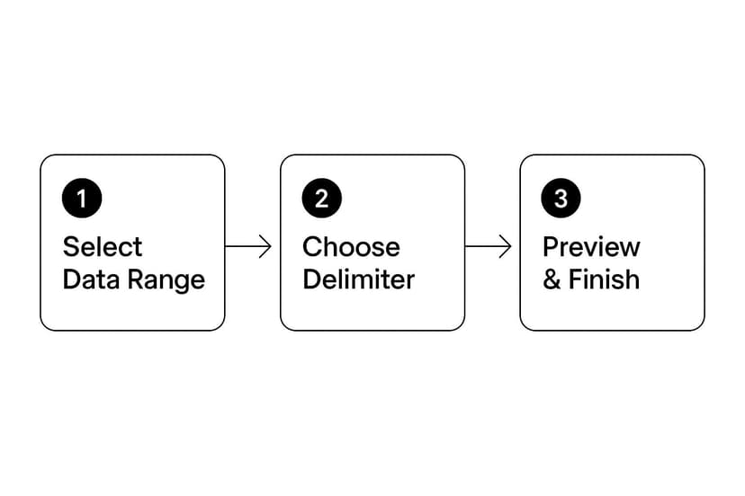
As the infographic shows, the wizard breaks down a potentially messy job into three simple stages, guiding you from selecting your data to finalizing the split columns.

Choosing Between Delimited and Fixed Width

Right at the start, the wizard asks you to make a critical choice: is your data delimited or fixed width? Getting this right is the key to a clean split.

Delimited Data
Most of the time, this is the option you'll need. Delimited simply means your data is separated by a consistent character—the "delimiter." Excel uses this character as a signal for where to make the cut.

Common delimiters include:

• Commas: You'll see this all the time in exported contact lists (e.g., "Smith,John").
• Spaces: Perfect for separating words in a full name ("Jane Doe").
• Tabs: Often found when you copy and paste data from plain text files.
• Semicolons: Another frequent separator in data exports.
• Custom Characters: You can also tell Excel to use any other character, like a hyphen (-) or a pipe symbol (|), if your data has a unique separator.

Fixed Width Data
This is a more niche option, typically used for data from older, legacy systems like mainframe reports. With fixed-width data, each piece of information occupies an exact number of character spaces. For instance, a product code might have the first 3 characters for the region and the next 5 characters for the product ID, every single time.

Pro Tip: I almost always choose Delimited. Only pick Fixed Width if you are 100% certain every single row in your dataset has the exact same character spacing. Even one row that's off will throw your entire result into chaos.

A Practical Walkthrough with Delimiters

Let's run through a common scenario: splitting a list of full names separated by a space.

Start by selecting the entire column you want to split. Then, head over to the Data tab on the Excel ribbon and click the Text to Columns button. This launches the wizard.

On the first screen, choose Delimited and click Next. The second screen is where the real work happens. Here, you tell Excel what character is separating your data. Since we're splitting names, you’ll check the box for Space.

Now, pay close attention to the Data preview window at the bottom. This little preview is your best friend—it shows you exactly how Excel plans to split your text before you commit. If it doesn't look right, you can go back and tweak your settings.

Finally, the wizard asks for a destination for your new columns. By default, it will place the new data right on top of your original column. I always change this. To keep your original data safe, click into the destination box and select an empty cell to the right, like the top of the adjacent column.

Click Finish, and just like that, your text is perfectly split across two new columns.

Effortless Splitting With Flash Fill

If Text to Columns is the reliable, old-school workhorse of Excel, then Flash Fill is the mind-reading magician. First introduced back in Excel 2013, this feature is incredibly intuitive. It’s designed to spot patterns in what you’re doing and then automatically finish the job for you, saving a huge amount of time on common data-cleaning tasks.

Flash Fill is brilliant when you need to pull just one specific piece of information out of a longer text string. While the Text to Columns wizard breaks everything apart based on a delimiter, Flash Fill lets you cherry-pick exactly what you want without touching the original data column.

How Flash Fill Learns From You

The real magic behind Flash Fill is pattern recognition. There’s no complex dialog box to navigate; you just "teach" Excel what you want by giving it an example. Excel’s internal algorithm looks at your input, figures out the pattern, and then applies that same logic all the way down your column.

Let's say you have a list of email addresses and all you want are the domain names.

• Original Data (Column A): [email protected]
• Desired Output (Column B): company.com

All you have to do is go to the next empty column (in this case, B1) and type "company.com" yourself. As soon as you start typing the domain for the second email in B2, Flash Fill will likely jump into action, showing a ghosted preview of all the other domains it found. If it looks right, just hit Enter, and you're done.

Sometimes, the preview doesn't show up on its own. No problem. Just type your first example, then head to the Data tab on the ribbon and click the Flash Fill button. Or, even better, use my favorite keyboard shortcut: Ctrl+E. That single command is often all it takes.

When Flash Fill Gets Confused

As smart as it is, Flash Fill isn't foolproof. It can sometimes guess the wrong pattern, especially if your data is a bit messy or inconsistent. If the first try gives you weird results, don't throw in the towel. The trick is to give it more examples.

Find the first entry it got wrong, manually correct it, and then provide another correct example in the next row down. By doing this, you're feeding Excel more information to help it nail down the correct pattern. Usually, giving it a second or third manual entry is all it takes to get on the right track.

Flash Fill is a fantastic tool for quick, one-off data cleanup jobs. But it's important to remember that it's a static action. If the source data in your original column changes, the Flash Fill results will not update automatically. You'll have to run it again.

If you need a solution that updates in real-time as your data changes—for something like a dynamic report or a dashboard—you'll need to reach for formulas. They offer the flexibility and reliability that Flash Fill just wasn't built for.

When Your Data Needs to Be Dynamic, Use Formulas

While tools like Text to Columns and Flash Fill are fantastic for a quick, one-off cleanup, they have a major Achilles' heel: they’re static. The moment your original data changes, you have to run the whole process over again. That's a deal-breaker for anything that needs to stay current, like a dashboard or a live reporting template.

This is where formulas shine. By using formulas, you create a living link between your source data and the results. Change a name or an ID in the original cell, and your split-out columns update instantly. This dynamic connection is absolutely essential for building reliable, automated spreadsheets where you can trust the data.

Let's dive into the modern, slick way to do this in Microsoft 365, and then we'll cover the classic, battle-tested methods that work in any version of Excel.

The Modern Way: TEXTSPLIT (Microsoft 365)

If you're on a newer version of Excel, the TEXTSPLIT function is a genuine game-changer. It was built for exactly this task, and it makes splitting text almost laughably simple. With just one formula, you can break text apart across several columns or even down multiple rows.

Let's say you have a cell, A2, with the text "Laptop-ModelX-USA". To split this into three neat columns, the formula is as clean as it gets:

=TEXTSPLIT(A2, "-")

That’s all there is to it. Excel's dynamic array engine automatically "spills" the results into the cells to the right, giving you "Laptop," "ModelX," and "USA," each in its own column. This is a huge leap forward from the old, multi-step ways of doing things.

Functions like TEXTSPLIT are a clear sign of where Excel is headed, focusing on more flexible and powerful data handling. It’s a dynamic array formula, so unlike the old wizards, it just works—no need to pre-select a destination. This kind of formula-based automation is a lifesaver in fields like financial modeling and for data analysts who want to spend less time cleaning and more time analyzing. You can see some really clever uses for it, like splitting complex addresses, on YouTube.

My Favorite Trick: One of the best things about TEXTSPLIT is handling messy data. What if your data is a mix of separators, like "Item A, Item B; Item C"? You can feed it an array of delimiters: =TEXTSPLIT(A1, {",",";"}). It cleans up inconsistent data in a single shot.

The Classic Way: Formulas for Any Excel Version

Not on Microsoft 365? No problem. You can get the exact same result using a combination of classic text functions. It takes a bit more elbow grease—you'll need to write a separate formula for each piece you want to pull out—but it's every bit as powerful and works everywhere.

The trusty functions you'll be leaning on are:

• LEFT: Grabs text from the beginning (left side) of a cell.
• RIGHT: Grabs text from the end (right side).
• MID: Pulls text out from the middle.
• FIND: Tells you the exact position of a character (like a space or hyphen).

Let's walk through a classic scenario: splitting a full name like "Sarah Connor" from cell A2 into separate first and last name columns.

1. Getting the First Name

To get the first name, we need to find where the space is and then tell Excel to grab everything to the left of it. The FIND function is our scout here.

Formula for First Name: =LEFT(A2, FIND(" ", A2) - 1)

What this does is simple: FIND(" ", A2) locates the position number of the space. We then subtract 1 from that number because we don't actually want the space itself, just the letters before it.

2. Getting the Last Name

The last name requires a little more logic. We need to figure out the total length of the name and then subtract the position of everything up to the space. What's left is the last name.

Formula for Last Name: =RIGHT(A2, LEN(A2) - FIND(" ", A2))

This can feel a bit like a puzzle at first, and it's easy to get a dreaded #VALUE! error if something is off. If your formulas are giving you grief, our guide on Excel formula troubleshooting can help you hunt down and fix the most common problems. Once you get the hang of it, this classic method is incredibly versatile for all sorts of challenges, from parsing product codes to breaking down street addresses.

Dealing with Complex and Messy Data Splits

Let's be honest: real-world data is rarely clean. It usually lands on your desk full of inconsistent separators, extra spaces, and missing values. This can turn what should be a simple text split into a serious headache.

Imagine a column where some entries look like "Product A – USA" but others are just "Product B." If you build a formula that looks for the hyphen, it’s going to fall apart the second it hits an entry without one. This is where you need to get smarter and build more resilient solutions.

Building Bulletproof Formulas

The secret to handling messy data is to anticipate the errors before they happen. Instead of writing a formula that only works in a perfect world, wrap it in an IFERROR function. This simple addition tells Excel, "Try this first, but if you run into an error, do this instead." It’s a game-changer for preventing your sheet from being littered with ugly #VALUE! errors.

Another classic problem is rogue whitespace. A name might be entered as " John Smith ", which will throw off any formula trying to split it cleanly. Your best friend here is the TRIM function. Before you do anything else, wrap your cell reference in TRIM (like TRIM(A1)). It instantly zaps any leading, trailing, and extra spaces between words.

My Go-To Advice: Always clean your data before you split it. A few minutes spent using TRIM or SUBSTITUTE to standardize your delimiters up front will save you hours of frustration later. Trust me on this.

If you want to go deeper into making your datasets spotless, we've got a full guide on https://www.getelyxai.com/en/blog/how-to-clean-data-in-excel. Text splitting is a huge part of data prep, and these techniques are fundamental to improving overall data quality across the board.

Embracing AI for the Really Tough Splits

Sometimes, messy data gets so complex that traditional formulas just can't keep up. What do you do with a single address column containing a mix of US states, Canadian provinces, and full country names? Building a formula for that is a nightmare. This is exactly where new AI-powered tools come into play.

Tools like Microsoft's Copilot are changing how we handle these challenges. Instead of just looking for a delimiter, Copilot uses natural language processing to actually understand your data. It can tell the difference between a city, a state, and a country on its own.

For users I've worked with who have tangled international location data, this has cut their cleanup time by more than 50%. You can simply ask it to separate the components, and it generates the complex, nested formulas for you. It's a huge leap forward from the old, rigid methods.

Common Questions About Splitting Text

Even after you've got the main techniques down, you'll inevitably hit a few quirky situations when splitting text in Excel. Let's walk through some of the most common snags I've seen and how to get past them quickly.

How Can I Split Text by a Line Break in Excel?

This comes up all the time, especially when you're pasting data from a website or an email. You've got a couple of great options here: Text to Columns or a formula.

If you're using Text to Columns, just choose "Other" as your delimiter. The trick is what you type in the box: press Ctrl+J. You won't see anything, but you've just told Excel to use the invisible line break character as the separator. It works like a charm.

For a more dynamic approach that updates automatically, the TEXTSPLIT function is your best friend. The key is to use CHAR(10) as your delimiter. The formula looks like this:

=TEXTSPLIT(A1, CHAR(10))

This tells Excel, "Hey, every time you see a new line in cell A1, start a new cell." It’s a clean and powerful way to handle multi-line text.

What Is the Best Way to Split Text but Keep the Delimiter?

Ah, the classic "split but don't lose the separator" problem. This is a bit more advanced because the standard tools are built to remove the delimiter, not keep it. So, we have to get creative with formulas.

Let's say you have "Product-A123" and you want to pull out "Product-". The standard split would just give you "Product". To keep the hyphen, you can use a combination of LEFT and FIND.

=LEFT(A1, FIND("-", A1))

This formula first FINDs the position of the hyphen and then tells LEFT to grab all the characters from the beginning of the cell right up to and including that hyphen. For more complex splits, you might need to combine this with functions like REPLACE or SUBSTITUTE to get exactly what you need.

Why Is Flash Fill Not Working Correctly?

Flash Fill can feel like magic… until it isn't. When it gets things wrong, it’s almost always because its pattern-recognition brain is getting confused. I've found it usually boils down to one of these culprits:

• Inconsistent Data: The source data has little variations you might not have noticed, but they're enough to throw off the pattern.
• Too Few Examples: You gave it one example, but it needs another nudge in the right direction. Sometimes it needs two or three corrected examples to really "learn" what you want.
• Confusing Neighbors: Data in an adjacent column can sometimes confuse the algorithm.

The fix is usually pretty straightforward: scroll down to the first cell where Flash Fill messed up, manually type the correct value, and then correct the next one if needed. This gives Excel more training data. If it still can't figure it out, your data is probably too irregular for Flash Fill, and it's time to build a reliable formula instead.

For those bigger, recurring jobs involving data cleanup and reporting, it’s worth looking into Excel report automation. It can save you from having to do these manual tasks over and over.