How to Analyze Data in Excel A Practical Guide

So, you've got a mountain of data sitting in a spreadsheet. What's next? The real magic happens when you start analyzing it—cleaning up the raw numbers, sorting and filtering to find what matters, using Pivot Tables to see the big picture, and creating charts that tell a compelling story. This process is the bedrock of business intelligence, turning confusing data into clear, confident decisions.

Why Excel Is Still Your Data Analysis Powerhouse

Before we jump into the "how," let’s talk about the "why." In a world flooded with specialized BI platforms, you might wonder if Excel is still relevant. The short answer is: absolutely. Its enduring power comes from a perfect mix of being incredibly accessible while having a surprisingly deep well of capabilities.

Just about every professional has access to Excel, which makes it a common language for sharing and working with data. This eliminates the friction of needing expensive, specialized software, allowing teams to collaborate seamlessly.

The Starting Point for Modern Analytics

For most of us, Excel is the first stop on any data journey. It's where raw data gets its initial "health check." You can run a quick sort to spot outliers, apply a filter to zero in on a specific product line, or build a simple chart to see if a trend is emerging. This initial exploration is a fundamental, and often overlooked, part of the process.

The numbers back this up. An estimated 750 million people use Excel globally. Even seasoned data scientists often turn to it for initial data cleaning and basic statistical work before moving to more complex tools. Its versatility keeps it right at the center of the analytics world. You can read more about why data pros still use Excel to see how it fits into their workflows.

My Take: Excel’s real strength isn't just a list of features, but its sheer ubiquity. It’s the common ground where data analysis begins for millions of people every single day.

To get a quick overview of the methods we'll be discussing, here's a simple table that breaks down the core techniques.

Core Excel Analysis Techniques at a Glance

Technique	Primary Use Case
Sort & Filter	Quickly organizing data and isolating specific subsets for review.
Formulas & Functions	Performing calculations, from simple arithmetic to complex statistical analysis.
Conditional Formatting	Highlighting cells with colors, icons, or data bars to visually spot trends.
Charts & Graphs	Creating visual representations of data to make it easy to understand.
Pivot Tables	Summarizing large datasets to uncover patterns and relationships interactively.
Power Query	Importing, cleaning, and transforming data from various sources automatically.

Each of these tools plays a specific role, and mastering them will give you a comprehensive toolkit for tackling any dataset.

More Than Just a Spreadsheet

Don't mistake today's Excel for the simple grid of cells it started as. It has grown into a seriously robust analysis tool with features that can handle massive data workloads, which is why it remains so competitive.

Here are a few of the game-changers:

Power Query: This is your data-cleaning workhorse. It lets you connect to different data sources, combine them, and automate the tedious prep work that used to take hours.
Pivot Tables: With a few clicks, you can summarize and reorganize millions of rows of data to see relationships you'd never spot otherwise—all without writing a single formula.
Dynamic Arrays: A more recent addition that totally changes the formula game. Now, a single formula can return a whole range of results, simplifying what used to be incredibly complex calculations.

As you learn to analyze data in Excel, you'll find that new tools like Elyx.AI can enhance these capabilities even further. For more tips on leveling up your data skills, you can always find fresh ideas on the Elyx.AI blog. This guide will give you the foundational steps to start your journey.

Turning Messy Data into a Clean Slate

Before you can even think about finding stories in your data, you have to get your hands dirty. It’s a lot like cooking—the most amazing recipe is useless if your ingredients are spoiled. This is the stage where great analysis begins, transforming a chaotic spreadsheet into a reliable foundation for discovery.

Rarely does data arrive perfectly packaged. More often than not, you'll find names and addresses smooshed into one cell, different labels for the same thing (like "USA" and "United States"), or duplicate rows from a botched export. If you ignore these little messes, they'll snowball, skewing your results and leading you to completely wrong conclusions.

The Essential Cleanup Toolkit

Your first pass at cleaning will likely involve a few classic Excel tools. I consider these non-negotiable skills for any analyst. They’re built right into Excel and designed to handle the most common data headaches you'll face. Getting comfortable with them is a huge part of learning how to analyze data in Excel.

Here are the tools I use all the time:

Text to Columns: This feature is an absolute lifesaver. Got a column with "Firstname Lastname" that you need to split? Text to Columns can separate it based on a space, comma, or any other delimiter in just a few clicks.
Remove Duplicates: You'll find this under the Data tab, and it does exactly what you'd expect. It scans your data and zaps any rows that are perfect copies of each other. This is crucial for getting accurate counts and unique records.
Find and Replace: This is your best friend for standardization. For example, you can instantly find every instance of "NY" and replace it with "New York," ensuring all your regional data gets grouped correctly later on in a Pivot Table.

You'll also want to keep an eye out for empty cells and incorrect data types. A blank cell can throw off your formulas, so you need a strategy—should you fill it with a zero, an "N/A," or something else? Likewise, make sure your numbers are actually stored as numbers, not text, or your calculations will fail.

Using AI to Fast-Track the Cleaning Process

Doing all this manually is fine for small files, but with thousands of rows, it becomes a soul-crushing time sink. This is exactly where an AI assistant comes in to save the day. Instead of clicking through endless menus and formulas, you can just tell the AI what you want in plain English.

Data cleaning isn't just about deleting things; it's about shaping your raw information into a trustworthy asset. The faster you get it done, the more time you have for the fun part—the actual analysis. An AI tool can slash this prep time.

For example, with an assistant like Elyx.AI, you can hand off complex cleaning jobs with a simple instruction.

Here’s a look at Elyx.AI in action, taking a simple command and tidying up a dataset automatically.

The AI is smart enough to spot the inconsistencies and make the right changes across your entire sheet. What would have taken you ages to do manually is done in seconds. This means you can get from messy spreadsheet to analysis-ready data in a fraction of the time.

Now that your data is clean and organized, it's time to dig in and find the story hidden within the numbers. For this, we turn to what is arguably Excel’s most powerful feature: the Pivot Table. If you've ever felt overwhelmed by a spreadsheet with thousands of rows, a Pivot Table is your best friend. It lets you condense all that raw data into a clear, meaningful summary without writing a single formula.

Think of it this way: a Pivot Table gives you a set of building blocks made from your data columns—things like "Sales," "Region," or "Product Category." You can then arrange and rearrange these blocks to see how they connect. For example, you can group all sales data by region in a matter of seconds. It's the fastest way to get from a wall of data to real answers.

Building Your First Interactive Report

Getting started is surprisingly straightforward. Just select your dataset, head to the Insert tab, and click PivotTable. Excel will then open a new sheet with a blank report on the left and a field list on the right. This is your canvas. You build your analysis by dragging fields into the four areas: Rows, Columns, Values, and Filters.

Want to see total sales for each product line? No problem. Drag your "Product" field to the Rows area and "Sales" to the Values area. Done. Curious which sales representative is crushing it this quarter? Drag "Sales Rep" to Rows, "Date" to Columns (Excel is smart enough to group dates automatically), and "Sales" back to Values. Every drag-and-drop action gives you a completely new view, letting you explore your data from different angles.

And it's not just about sums. With a quick right-click, you can switch from a total count to an average, find the maximum value, or pinpoint the minimum. This flexibility is precisely why anyone who works with data in Excel needs to master Pivot Tables.

A common hang-up I see is people thinking they need a perfect, fully-formed question before they even start. Forget that. The real magic of a Pivot Table is in the exploration. Just start dragging fields around and see what patterns jump out. Let the data itself spark your curiosity.

The infographic below really drives home how you can turn a spreadsheet of raw numbers into compelling charts that tell a clear story.

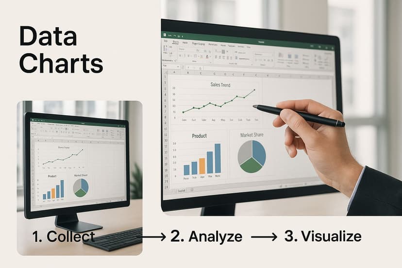
As you can see, it’s all about transforming raw inputs into visualizations that immediately highlight key business trends.

Let AI Create Your Pivot Tables

While building Pivot Tables by hand is a fundamental skill, what if you could just ask for the report you need? That's where AI assistants like Elyx.AI come into play. Instead of the usual drag-and-drop process, you can simply type a request in plain English, like, "Create a Pivot Table showing average customer satisfaction scores by service agent." The AI gets to work, interprets your request, and builds the entire table for you.

This approach makes one of Excel's most essential tools much more approachable, especially if you're just starting your data analysis journey. It's a game-changer.

The difference between the traditional method and an AI-powered one can be quite stark. Here’s a quick comparison of the steps involved:

Manual Pivot Table Creation vs AI-Assisted Generation

Action	Manual Excel Process	Elyx.AI Process
Initiation	Go to Insert > PivotTable. Confirm data range.	Open Elyx.AI. Type your request in the chat.
Layout	Drag "Region" to Rows. Drag "Product" to Columns.	The AI automatically places fields based on your prompt.
Calculation	Drag "Sales" to Values. Right-click to change from SUM to AVERAGE.	Specify "average sales" in your prompt. The AI sets the calculation.
Refinement	Manually add filters or slicers for "Year."	Refine by typing a follow-up: "Now filter for 2023 only."
Time	Can take several minutes, depending on complexity and familiarity.	Typically completed in under a minute.

As the table shows, AI doesn't just speed things up; it simplifies the entire thought process, letting you focus on the insights rather than the mechanics.

The demand for these analytical skills is exploding. Global spending on analytics software, which includes spreadsheet tools like Excel, recently reached an estimated USD 10.35 billion. This massive investment underscores how much companies value people who can turn data into decisions. You can learn more about the booming market for data analysis tools and see just how valuable your skills are becoming.

Going Deeper with Advanced Formulas

Once you have your data clean and summarized, formulas are what will take your analysis from good to great. Sure, Pivot Tables are fantastic for getting that bird's-eye view, but formulas let you get into the weeds and ask very specific, nuanced questions. This is where you graduate from basic sums and averages to uncovering the real stories buried in your spreadsheet.

The trick is learning how to chain functions together to build powerful, custom calculations. Mastering this is fundamental to learning how to analyze data in Excel because it gives you total control. You can precisely segment customers, automatically flag outliers, or stitch different datasets together.

Using Logic to Segment Your Data

At the core of any advanced analysis, you'll find logical functions. These are the tools that let you apply rules and conditions, acting like traffic cops for your data and directing calculations based on the criteria you set.

You'll find yourself returning to a few key logical functions again and again:

IF: This is your bread and butter. It simply checks if a condition is true and gives you one result if it is, and another if it isn't. For example, you could create a new column to segment orders with a formula like IF(B2>1000, "High Value", "Standard").
AND/OR: Think of these as partners to your IF function. You use them inside an IF to test multiple things at once. AND needs every condition to be true, while OR just needs one.
SUMIF/COUNTIF: These are incredibly handy for quick summaries without the hassle of a full Pivot Table. Need to know how many sales came from the "East" region? COUNTIF is your answer.

When you start combining these, you can create some really sophisticated segments. For instance, you could flag "high-priority leads" by checking if their lead score is above a certain number AND if their last contact was more than 30 days ago. That’s the kind of actionable insight that drives business decisions.

Merging Datasets with Lookup Functions

One of the most frequent—and sometimes frustrating—tasks in data analysis is combining information from different tables. You might have a sales table with a CustomerID but need the actual customer names and locations from a separate customer table. To analyze sales by region, you have to bring that data together.

For a long time, VLOOKUP was the default tool for this job, but frankly, it’s a bit clumsy. Its biggest drawback is that it can only look up data from left to right. A much more powerful and flexible method is to use a combination of INDEX and MATCH. This dynamic duo can pull data from any column, won't break if you add or remove columns later, and performs much faster on large datasets.

I tell everyone this: While VLOOKUP is easier to learn initially, taking the time to master INDEX/MATCH is one of the best investments you can make in your Excel skills. It truly opens up a new level of analytical power and is what separates casual users from the pros.

The formula might look a little intimidating at first, but its logic is simple. MATCH finds the row number for the item you're looking for, and INDEX then grabs the data from that specific row in the column you actually need.

With modern tools like Elyx.AI, you don't even have to sweat the syntax. You can just describe what you need in plain English. For example, asking the AI to "calculate the average order value for customers in the West region who purchased after June 1st" will spit out the perfect, error-free formula in seconds.

Here's a look at the Elyx.AI formula generator doing its thing.

This is a game-changer. It lets you skip the steep learning curve of complex functions and jump straight to getting answers. The best part is that the AI doesn't just write the formula; it also explains how it works, so you're actually learning as you go.

Bringing Your Data to Life with Visuals

Numbers on a spreadsheet can tell you what happened, but a good chart is what makes people feel the story. This is where your hard work of cleaning and analyzing data pays off. Turning those clean numbers into a clear, compelling visual is often the most critical step. It’s the difference between your findings being understood and your findings being ignored.

The real trick is picking the right tool for the job. You wouldn't use a hammer to saw a board, and you shouldn't use a pie chart to show a trend.

Are you comparing distinct items, like sales figures across different product lines? A bar chart is your go-to. It’s classic for a reason.
Need to illustrate how something has changed over time, like your website traffic over the last year? A line chart is perfect for showcasing trends and patterns.
Wondering if two different things are related, like how your advertising budget affects new customer sign-ups? A scatter plot is fantastic for uncovering potential relationships that are nearly impossible to spot in a table of numbers.

Designing Charts That Actually Communicate

Anyone can click "Insert Chart" in Excel. The real skill lies in creating a chart that someone can understand in five seconds or less. If your audience has to squint and struggle to figure out your point, you’ve already lost their attention.

Here are a few practical pointers I've learned over the years to keep my charts clean, professional, and instantly understandable:

Tell a Story with Your Title: Ditch generic labels like "Sales Data." Instead, frame the conclusion. A title like "Q3 Sales Growth Smashes Projections by 20%" immediately tells the viewer the key takeaway.
Use Color with Purpose: Color shouldn't just be for decoration; it should guide the eye. Use a single, strong color to highlight the most important data series and keep everything else in more muted, neutral tones. This creates a clear focal point.
Label Everything Clearly: Don't make people guess. Make sure your axes are labeled with the correct units (e.g., "Revenue in USD," "Number of Users"). Sometimes, adding data labels directly onto the bars or points on a chart is far more effective than forcing people to trace lines back to an axis.

The demand for people who can do this well is exploding. The global data analytics market, which was valued at around USD 48.53 billion, is on track to hit a staggering USD 329.13 billion by 2033. That massive growth shows just how much businesses need professionals who can not just crunch numbers, but effectively communicate what they mean. You can discover more insights about the data analytics market to see just how fast this field is moving.

Pro Tip: Stop manually rebuilding your charts every month. Instead, create dynamic charts that update themselves. Base your chart on a named Excel Table or a PivotTable. When you add new rows of data to your source table and hit 'Refresh,' your chart will instantly update with the latest information. This simple trick turns a static report into a living dashboard.

This approach is a huge time-saver. If you want to make things even more efficient, AI tools can seriously speed up how you analyze data in Excel. An AI assistant can handle many of the preliminary steps, like generating the summaries or PivotTables that your dynamic charts are built on.

If you're curious about how AI can help, consider grabbing a free download of the Elyx.AI add-in to see it in action.

Common Excel Analysis Questions Answered

Once you start getting the hang of analyzing data in Excel, you'll inevitably hit a few common snags. I like to think of these as rites of passage for any analyst. Let's walk through some of the questions I hear most often and give you some practical, real-world answers.

One of the biggest debates I see online and in training sessions is about lookup functions. Should you just use the classic VLOOKUP, or is it worth the effort to learn the more powerful INDEX/MATCH combination?

My take is simple: learn INDEX/MATCH. While VLOOKUP is fine for a quick and dirty lookup, its weaknesses show up fast. It can only look to the right of your lookup value, and the whole thing breaks if you dare to add or remove a column in your source data.

INDEX/MATCH, on the other hand, is built for flexibility. It can pull data from any column, doesn't care if you restructure your table, and frankly, it runs faster on large datasets. Putting in the time to master this duo will save you countless headaches down the road.

Dealing with Annoying Formula Errors

Nothing ruins a beautiful analysis faster than a spreadsheet filled with ugly errors like #N/A, #DIV/0!, or #VALUE!. They don't just look sloppy; they can completely break your summary calculations, like sums and averages. So, what's the fix?

The most elegant way to handle this is with the IFERROR function. Think of it as a safety net for your formulas. You just wrap your original formula inside of it and tell Excel what you want to see if an error pops up.

For instance, instead of a standard lookup that might fail:
=VLOOKUP(A2, SalesData, 2, FALSE)

You can build in a fallback like this:
=IFERROR(VLOOKUP(A2, SalesData, 2, FALSE), "Not Found")

Just like that, any failed lookups now show a clean "Not Found" message instead of a jarring error code. This keeps your data tidy and ensures your other calculations don't break.

How to Analyze Data from Multiple Sheets

Another challenge that comes up all the time is trying to pull together information from different worksheets. Let's say you have sales data split out by month—one tab for January, one for February, and another for March. How do you analyze it all together? You've got a couple of solid options here.

For Formulas: If your sheets are set up identically, you can use what's called a 3D reference. A formula like =SUM(Jan:Mar!B2) is a quick way to add the value from cell B2 across all three of those sheets.
For Pivot Tables: The better, more robust method is to use Power Query. It's designed for this exact scenario and can easily stack the data from multiple sheets (or even different files) into one master table. That clean, combined table is the perfect foundation for a powerful Pivot Table.

Wrangling these more complex functions can be tricky at first. If you ever get stuck or just need a clear walkthrough of a specific process, you can find detailed guides in the Elyx.AI help center, which is packed with step-by-step support for these kinds of Excel challenges.

Ready to stop wrestling with complicated formulas and manual data cleaning? Elyx.AI integrates directly into your spreadsheet, letting you generate insights, create Pivot Tables, and clean data with simple, plain-English commands. See how much faster you can work by visiting https://getelyxai.com and trying it for yourself.

Article created using Outrank