What Is VLOOKUP in Excel? A Practical Guide

If you've ever wasted time manually searching through a massive spreadsheet for a single piece of information, you understand the frustration. This is the exact problem VLOOKUP was designed to solve. It’s one of Excel's most powerful functions for linking related data between different tables.

Imagine you have a friend's name and need to find their phone number in your contacts. You would scan down the "Name" column, find their name, and then look across to the "Phone Number" column. VLOOKUP automates that exact process within your spreadsheet, delivering the result in a fraction of a second. This guide will provide practical, real-world examples to help you master this essential Excel skill.

Your Quick Guide to VLOOKUP in Excel

VLOOKUP stands for Vertical Lookup. The name itself describes its function: it scans vertically down the first column of a data table to find a specific value you provide.

Once it finds a match, it moves horizontally to the right along that same row to retrieve a piece of information from a column you specify. This is incredibly useful when you have two separate lists sharing a common identifier—like a product SKU or an employee ID—and you need to pull data from one list into the other.

Understanding the VLOOKUP Formula

To use VLOOKUP effectively, you need to understand its four components, known as arguments. Each argument is a precise instruction that tells the function what to find, where to look, and what information to return. Mastering these arguments is the key to making the formula work reliably every time.

If you're new to formulas, consider starting with our detailed guide on foundational Excel formulas for beginners.

The formula's structure is:

=VLOOKUP(lookup_value, table_array, col_index_num, [range_lookup])

Let's break down what each argument means. The table below offers a quick overview, followed by practical examples that show how they work together to solve real problems.

VLOOKUP Syntax At a Glance

Argument	What It Means	Example
lookup_value	The specific piece of information you are trying to find.	A product ID like "A-102"
table_array	The entire range of cells where your data lives. VLOOKUP always searches in the first column of this range.	A table from cell A2 to D50, written as A2:D50
col_index_num	The number of the column that contains the answer you want. The count starts from the left of your table_array.	The number 3 to get data from the 3rd column
[range_lookup]	Tells Excel if you want an exact match (FALSE) or an approximate match (TRUE).	FALSE (You'll use this 99% of the time!)

Getting comfortable with these four parts is the first major step. Once you understand their roles, you can start building powerful formulas to automate your work and save valuable time.

Breaking Down the VLOOKUP Formula

To truly master VLOOKUP, you need to understand the four key pieces of information it requires. Think of them as four simple instructions you give Excel to fetch exactly what you need. Get these four parts right, and you'll be able to automate searches that would otherwise take ages.

The formula itself looks like this:
=VLOOKUP(lookup_value, table_array, col_index_num, [range_lookup])

This simple infographic gives you a great visual of how VLOOKUP works. It shows the formula taking one piece of information, scanning a table for it, and then pulling out a related detail.

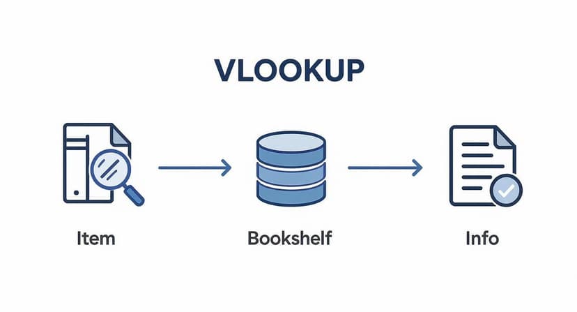
As you can see, the process is logical. The formula acts as a bridge, connecting the data you have to the data you need.

The Four Essential Arguments

Let's walk through each piece of the formula one by one.

• lookup_value: This is the value you are looking for. It's the piece of data you already possess, such as a product code, a customer ID, or an employee's name. This serves as your starting point.

• table_array: This is the range of cells that contains your data. It's the entire table Excel needs to search. The most critical rule to remember is that the column containing your lookup_value must be the first column in this range. For instance, if you're searching by product ID, the ID column must be the first one you select.

A quick pro-tip: Always use absolute references for your table (e.g., $A$2:$D$50 instead of A2:D50). This "locks" the table in place, preventing errors when you copy or drag your formula to other cells.

• col_index_num: This number tells VLOOKUP which column to retrieve the result from. Simply count from left to right, starting with your lookup column as 1. If you want to get the price from the third column in your table, you would enter 3.

• [range_lookup]: This final argument tells Excel whether you need an exact match or an approximate one. You have two options: FALSE for an exact match (e.g., finding a specific invoice number) or TRUE for an approximate match (e.g., finding a tax rate within an income bracket). In real-world applications, you will almost always use FALSE because you typically need the exact piece of data.

VLOOKUP, short for 'vertical lookup,' has been a game-changer in Excel since the late 1980s. Before it came along, finding information in a large spreadsheet meant a lot of scrolling and manual searching, which was slow and a recipe for mistakes. If you're curious about the backstory, you can explore this detailed video on VLOOKUP's origins.

Putting VLOOKUP to Work with Real Examples

Theory is one thing, but seeing VLOOKUP solve actual problems is where its value becomes clear. Let’s explore three common scenarios that demonstrate how this single formula can eliminate tedious, error-prone manual data entry.

Example 1: Find an Employee's Department

Imagine you have a list of new hires and need to identify their departments. You have their Employee IDs, but the department information is located in a large, master employee database on another worksheet.

Here’s what your two tables might look like:

New Hires (Your destination table)

Employee ID	Name	Department
104	David Chen	?

Master Employee List (Your source data)

Employee ID	Full Name	Department
101	Sarah Smith	Marketing
102	John Doe	Sales
103	Emily Jones	Engineering
104	David Chen	Finance

To automatically find David's department, you would use this formula:
=VLOOKUP(104, MasterListRange, 3, FALSE)

Excel takes the ID 104, finds it in the first column of your master list, moves to the third column, and returns the value it finds: "Finance." This is incredibly useful for tasks like managing timesheets in Excel, where you constantly need to consolidate related information.

Example 2: Combine Sales Data

Here’s another classic scenario. You have a worksheet with daily sales, containing only Product IDs and the quantity sold. To calculate revenue, you need to pull in the price for each item from your master product catalog.

This is a perfect job for VLOOKUP:

• What to look for: The Product ID from your daily sales sheet.
• Where to look: Your entire product catalog, making sure Product IDs are in the first column.
• What to bring back: The column with the price (let's say it's column 2).
• How to look: FALSE, because you need an exact match for each product.

The formula =VLOOKUP(ProductID, ProductCatalog, 2, FALSE) will instantly fetch the correct price for every single item, saving you from manual lookups.

Example 3: Assign Grades with an Approximate Match

Finally, let's look at a practical case for using the TRUE argument for an approximate match. A teacher wants to assign letter grades based on numeric test scores.

First, create a grading scale table, sorted in ascending order by score.

Grading Scale (Sorted smallest to largest)

Score	Grade
0	F
60	D
70	C
80	B
90	A

If a student scores an 85, the formula =VLOOKUP(85, GradingScale, 2, TRUE) finds the correct grade. It scans the Score column for the largest value that is less than or equal to 85. It finds 80, looks to the second column, and returns the grade "B." This is one of the most powerful and common use cases for the TRUE argument.

Solving Common VLOOKUP Problems

It's a common experience: you construct what seems like a perfect VLOOKUP formula, press Enter, and an error appears. This is a normal part of learning any new Excel function.

Think of these errors as helpful clues rather than obstacles. Each error code is Excel's way of telling you precisely what went wrong. Once you learn to interpret them, fixing formulas becomes straightforward. Let's break down the most common VLOOKUP errors you'll encounter.

Decoding the #N/A Error

The #N/A error is the most frequent one. It stands for "Not Available," meaning Excel searched for your item in the first column but couldn't find it.

• What It Means: The value you're looking for does not exist in the lookup list. This is often caused by a simple typo, an extra space at the end of a cell, or because the data is genuinely missing.
• How to Fix It: First, double-check your lookup value for spelling mistakes or hidden spaces. If the data is correct but you want to present a cleaner result, you can wrap your VLOOKUP in an IFERROR function. For example, =IFERROR(VLOOKUP(...), "Not Found") will display a user-friendly message instead of the error.

Why You See the #REF! Error

Another common error is #REF!. This indicates an invalid cell reference, meaning your formula is pointing to a location that doesn't exist.

The most common cause of a #REF! error is requesting a column number that is outside your table's range. For example, telling VLOOKUP to return the 5th column from a table that only has 4 columns will always trigger this error.

The solution is typically simple: ensure your column index number is within the bounds of your selected table. For more general advice, our guide on how to approach Excel formula troubleshooting is an excellent resource.

Quick Guide: Troubleshooting Common VLOOKUP Errors

A quick reference can be invaluable when troubleshooting. This table breaks down common VLOOKUP errors, their causes, and actionable solutions.

Error Code	Common Cause	How to Fix It
#N/A	The lookup value doesn't exist in the first column of the table.	Check for typos or extra spaces. Use IFERROR to display a custom message.
#REF!	The col_index_num is greater than the number of columns in the table_array.	Adjust the column index number to be within the valid range of your table.
#VALUE!	The col_index_num is less than 1 or contains text.	Ensure the column index is a positive number.
Wrong Result	You're using TRUE for an approximate match on an unsorted list.	Sort your lookup column in ascending order or switch to FALSE for an exact match.

Keep this table handy as your cheat sheet for resolving VLOOKUP issues.

Other Common VLOOKUP Mistakes

Beyond specific error codes, a few other mistakes can cause problems. If you're getting an incorrect result without an error, you might have duplicate values in your lookup column. Remember, VLOOKUP always stops at the first match it finds and ignores any subsequent ones.

Another frequent oversight is forgetting to lock your table_array with absolute references (e.g., $A$2:$D$50). Without the dollar signs, the table range will shift as you copy the formula down, leading to incorrect results and errors. Always lock your table to ensure it remains fixed on the correct data source.

When VLOOKUP Is Not Enough

Despite its power, VLOOKUP has limitations. Understanding its weaknesses is the first step toward becoming a true data lookup expert in Excel.

VLOOKUP’s biggest drawback is its inability to look to the left. The value you're searching for must be in the first column of your specified range. It's a one-way street.

Furthermore, it can become slow when working with very large datasets. Perhaps most frustratingly, if you insert a new column into your source table, any VLOOKUP formulas pointing to it will break because the column index number becomes incorrect. When you encounter these issues, it's a sign that it's time to explore more modern and flexible tools.

Modern Alternatives to VLOOKUP

Fortunately, Excel has evolved. For years, the standard workaround for VLOOKUP's limitations was a combination of two functions: INDEX and MATCH. This pair is far more flexible, as it can look up data in any direction—left, right, up, or down—and it doesn't break when columns are added or removed.

However, a superior solution now exists: XLOOKUP, available in newer versions of Excel. It was designed specifically to address VLOOKUP's shortcomings. It features a simpler syntax, can look in any direction by default, and defaults to an exact match, which is safer. Crucially, it is not affected by the insertion or deletion of columns.

You might think VLOOKUP is on its way out, but it’s still everywhere—especially in finance. Surveys show that over 70% of finance professionals still rely on it for things like matching up transaction data. Millions of people search for how to use it every year, which just goes to show how essential it remains.

For a deeper dive into why it's still so prevalent, you can explore more about its continued relevance on corporatefinanceinstitute.com.

Here's a quick video that walks you through why XLOOKUP is often the better choice:
https://www.youtube.com/embed/Gfu26nNvrsk

When dealing with datasets so large they slow Excel to a crawl, you need a more robust system. For complex scenarios, it's beneficial to understand the fundamentals of data pipelines. If you want to stay within the Excel ecosystem but require more power, Power Query is the answer. Our guide on getting started with Power Query can help you get started.

VLOOKUP FAQs

Even after you get the hang of VLOOKUP, some common questions tend to pop up. Nailing down these details will save you a ton of headaches later and really cement your understanding of how Excel's lookup functions work.

Why Is My VLOOKUP Not Working With Numbers?

This is a classic snag, and it almost always boils down to a formatting mismatch. To you, 123 is the same as 123, but Excel might see one as a true number and the other as text. VLOOKUP needs an exact match—including the data type—so it won't see those two as the same.

The fix is to make sure your lookup value and the first column of your data are formatted identically. You can do this by highlighting the cells, right-clicking to select Format Cells, or by using functions like VALUE() or TEXT() to force a conversion.

Can VLOOKUP Return Multiple Results?

In a word, no. VLOOKUP is designed to stop as soon as it finds the first match in your data. If you have duplicate lookup values, it will only return the result for the very first one it stumbles upon and ignore the rest.

If you need to pull all matching records, you’ll want to look at a more modern function like FILTER.

Key Takeaway: Think of VLOOKUP as a "one-and-done" function. It finds the first match, grabs the corresponding data, and its job is over.

Should I Still Use VLOOKUP Instead of XLOOKUP?

For any new spreadsheet, XLOOKUP is the superior choice. It’s more powerful, less prone to errors, and simpler to use.

So why bother learning VLOOKUP? Compatibility. It is still prevalent in legacy workbooks and is essential when collaborating with individuals using older versions of Excel. Knowing how to use VLOOKUP remains a valuable, practical skill for navigating the real world of shared spreadsheets.

---

Ready to stop wrestling with formulas and let AI handle the heavy lifting? Elyx.AI integrates directly into your spreadsheet, allowing you to clean data, generate complex formulas, and get insights just by asking. Transform your Excel workflow by visiting https://getelyxai.com and see what you can accomplish.